Writing Your First Quantum Circuit with Qiskit

Table of Contents

1. Introduction
2. What Is a Quantum Circuit?
3. Prerequisites for Running a Circuit
4. Installing and Importing Qiskit
5. Building a Basic Quantum Circuit
6. Commonly Used Quantum Gates
7. Applying Quantum Gates Step-by-Step
8. Visualizing the Circuit
9. Adding Measurements to Qubits
10. Choosing a Backend (Simulator vs Real Device)
11. Executing the Circuit on a Simulator
12. Viewing and Interpreting Results
13. Running the Circuit on IBM Quantum Hardware
14. Using Qiskit Tools for Circuit Analysis
15. Saving and Reusing Circuits
16. Tips for Beginners
17. Common Errors and How to Fix Them
18. Expanding to Multi-Qubit Circuits
19. Sample Exercises
20. Conclusion

1. Introduction

Creating your first quantum circuit is an exciting step toward understanding and using quantum computers. This guide uses Qiskit to walk you through building, visualizing, and running a simple quantum circuit.

2. What Is a Quantum Circuit?

A quantum circuit is a sequence of quantum gates applied to qubits. It’s the quantum analog of a classical logic circuit, but with reversible and probabilistic behavior.

3. Prerequisites for Running a Circuit

• Python 3.7 or later
• Qiskit installed (pip install qiskit)
• Optional: Jupyter Notebook for an interactive experience

4. Installing and Importing Qiskit

pip install qiskit

In Python:

from qiskit import QuantumCircuit, Aer, execute

5. Building a Basic Quantum Circuit

qc = QuantumCircuit(2, 2)  # 2 qubits, 2 classical bits

This initializes a circuit with 2 qubits and 2 classical bits for measurement results.

6. Commonly Used Quantum Gates

• X: Pauli-X (NOT)
• H: Hadamard (superposition)
• CX: CNOT (entanglement)
• Z, Y, S, T: phase and rotation gates

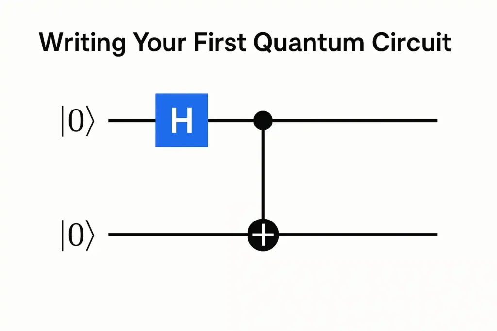
7. Applying Quantum Gates Step-by-Step

qc.h(0)      # Apply Hadamard gate to qubit 0
qc.cx(0, 1)  # Apply CNOT with control=0, target=1

8. Visualizing the Circuit

print(qc.draw())

Or in Jupyter:

qc.draw('mpl')

9. Adding Measurements to Qubits

qc.measure([0, 1], [0, 1])  # Measure qubit 0 into bit 0, qubit 1 into bit 1

10. Choosing a Backend (Simulator vs Real Device)

Use the Aer simulator for fast testing:

simulator = Aer.get_backend('qasm_simulator')

11. Executing the Circuit on a Simulator

job = execute(qc, simulator, shots=1024)
result = job.result()
counts = result.get_counts(qc)
print(counts)

12. Viewing and Interpreting Results

from qiskit.visualization import plot_histogram
plot_histogram(counts)

This shows the probability distribution over measured outcomes.

13. Running the Circuit on IBM Quantum Hardware

from qiskit_ibm_provider import IBMProvider
provider = IBMProvider()
backend = provider.get_backend('ibmq_qasm_simulator')
job = execute(qc, backend, shots=1024)

14. Using Qiskit Tools for Circuit Analysis

from qiskit.transpiler import PassManager
from qiskit.transpiler.passes import Depth
pm = PassManager(Depth())
print(pm.run(qc))

15. Saving and Reusing Circuits

qc.qasm(filename="my_first_circuit.qasm")

Or save with Python pickle:

import pickle
with open("my_circuit.pkl", "wb") as f:
    pickle.dump(qc, f)

16. Tips for Beginners

• Start with 1-2 qubit circuits
• Use simulators before real devices
• Explore gates visually
• Experiment with different combinations

17. Common Errors and How to Fix Them

• Missing measurements → No classical result
• Backend not found → Check Aer or IBM setup
• API error → Verify IBM token and internet

18. Expanding to Multi-Qubit Circuits

Try:

qc = QuantumCircuit(3, 3)
qc.h(0)
qc.cx(0, 1)
qc.cx(1, 2)
qc.measure([0,1,2], [0,1,2])

19. Sample Exercises

• Create a Bell state and verify entanglement
• Implement a Deutsch-Jozsa algorithm
• Simulate Grover’s algorithm with 2 qubits

20. Conclusion

Writing your first quantum circuit opens the door to a new computing paradigm. Using Qiskit, you can simulate, analyze, and eventually run your circuits on real quantum processors.