


Home Blog Page 287

Infinite Potential Well: Quantization in a Box

0
infinite potential well

Table of Contents

  1. Introduction
  2. Concept of the Infinite Square Well
  3. Mathematical Formulation
  4. Schrรถdinger Equation Inside the Well
  5. Boundary Conditions and Wavefunction Form
  6. Quantized Energy Levels
  7. Normalized Wavefunctions
  8. Probability Distributions and Nodes
  9. Expectation Values and Uncertainty
  10. Comparison with Classical Mechanics
  11. Time Evolution of Superpositions
  12. 3D Infinite Potential Well
  13. Applications in Nanotechnology and Quantum Dots
  14. Idealization and Realistic Potentials
  15. Conclusion

1. Introduction

The infinite potential well, also known as the particle in a box, is one of the most fundamental models in quantum mechanics. It exemplifies how quantum confinement leads to energy quantization, and is a cornerstone for understanding more complex systems like atoms, molecules, and quantum wells in nanotechnology.


2. Concept of the Infinite Square Well

  • A particle is confined between two impenetrable walls at \( x = 0 \) and \( x = L \)
  • The potential \( V(x) \) is defined as:

\[
V(x) = \begin{cases}
0, & 0 < x < L \
\infty, & \text{otherwise}
\end{cases}
\]

  • The particle is strictly confined in the region \( (0, L) \)

3. Mathematical Formulation

Inside the well, the time-independent Schrรถdinger equation is:

\[
\frac{\hbar^2}{2m} \frac{d^2\psi(x)}{dx^2} = E \psi(x)
\]

Outside the well, \( \psi(x) = 0 \) due to the infinite potential.


4. Schrรถdinger Equation Inside the Well

Define:

\[
k^2 = \frac{2mE}{\hbar^2}
\]

The general solution inside the well is:

\[
\psi(x) = A \sin(kx) + B \cos(kx)
\]

Apply boundary conditions to determine constants.


5. Boundary Conditions and Wavefunction Form

  • At \( x = 0 \), \( \psi(0) = 0 \) โ‡’ \( B = 0 \)
  • At \( x = L \), \( \psi(L) = 0 \) โ‡’ \( \sin(kL) = 0 \)

So:

\[
k = \frac{n\pi}{L}, \quad n = 1, 2, 3, \dots
\]

Thus, wavefunctions are:

\[
\psi_n(x) = A_n \sin\left( \frac{n\pi x}{L} \right)
\]


6. Quantized Energy Levels

Plug \( k \) into energy expression:

\[
E_n = \frac{n^2 \pi^2 \hbar^2}{2mL^2}
\]

Key features:

  • Discrete, non-zero ground state energy
  • Increases with \( n^2 \)
  • No degeneracy in 1D

7. Normalized Wavefunctions

Normalization condition:

\[
\int_0^L |\psi_n(x)|^2 dx = 1
\]

Gives:

\[
\psi_n(x) = \sqrt{\frac{2}{L}} \sin\left( \frac{n\pi x}{L} \right)
\]

Each \( n \) corresponds to a unique eigenstate.


8. Probability Distributions and Nodes

  • \( |\psi_n(x)|^2 \) gives probability density
  • Number of nodes = \( n – 1 \)
  • Higher \( n \): more oscillatory behavior

Expectation values:

\[
\langle x \rangle = \frac{L}{2}, \quad \langle x^2 \rangle = \frac{L^2}{3} – \frac{L^2}{2\pi^2 n^2}
\]


9. Expectation Values and Uncertainty

Uncertainty in position:

\[
\Delta x = \sqrt{\langle x^2 \rangle – \langle x \rangle^2}
\]

Increases with \( n \), but still bounded due to confinement.


10. Comparison with Classical Mechanics

  • Classical particle has uniform probability across the well
  • Quantum particle has non-uniform, oscillating probability
  • As \( n \to \infty \), quantum distribution approaches classical (correspondence principle)

11. Time Evolution of Superpositions

General state:

\[
\Psi(x,t) = \sum_n c_n \psi_n(x) e^{-iE_n t/\hbar}
\]

  • Leads to quantum beating, revivals, and interference
  • Time-dependence arises from phase factors \( e^{-iE_n t/\hbar} \)

12. 3D Infinite Potential Well

For a cubic box of size \( L \):

\[
\psi_{n_x,n_y,n_z}(x,y,z) = \left( \frac{2}{L} \right)^{3/2} \sin\left( \frac{n_x \pi x}{L} \right) \sin\left( \frac{n_y \pi y}{L} \right) \sin\left( \frac{n_z \pi z}{L} \right)
\]

\[
E = \frac{\pi^2 \hbar^2}{2mL^2} (n_x^2 + n_y^2 + n_z^2)
\]

Degeneracy occurs for states with same \( n_x^2 + n_y^2 + n_z^2 \).


13. Applications in Nanotechnology and Quantum Dots

  • Electrons in quantum wells and nanostructures behave like particles in boxes
  • Infinite well approximates confinement in thin films and quantum dots
  • Optical properties and energy levels are engineered using well geometry

14. Idealization and Realistic Potentials

  • Infinite well is an ideal model
  • Real systems have finite potential barriers
  • Leads to tunneling, resonance, and bound states with leakage

Still, infinite wells give excellent qualitative insight.


15. Conclusion

The infinite potential well offers a crystal-clear example of quantum confinement, discrete energy levels, and wavefunction behavior. Though idealized, it forms the basis of quantum mechanics education and inspires real-world applications in nanophysics, photonics, and quantum computing. It captures the essence of quantization โ€” the idea that even free particles can only exist in discrete energy states due to boundary conditions.


.

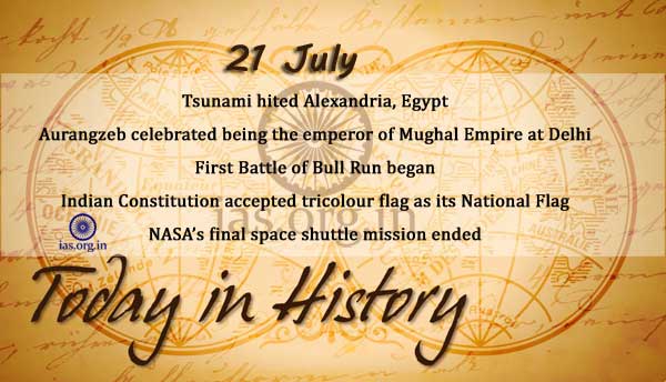
Today in History – 21 July

1
today in history 21 july

today in history 21 july

365

On this day in the year 365, a powerful earthquake off the coast of Greece caused a tsunami that devastated the city of Alexandria, Egypt. Although there were no measuring tools at the time, scientists now estimate that the quake was actually two tremors in succession, the largest of which is thought to have had a magnitude of 8.0.

1658

Aurangzeb celebrated being the emperor of Mughal Empire at Delhi. He was informally enthroned.

1861

In the first major land battle of the Civil War, a large Union force under General Irvin McDowell troops along the Bull Run stream in Virginia was routed by a Confederate army under General Pierre G.T. Beauregard.

1891

Jairamdas Doulatram, great leader, journalist and freedom fighter, was born at Karachi.

1906

W.C. Bonerjee, first President of Indian National Congress, passed away.

1935

Establishment of ‘Mumabi Marathi Sahitya Sangh’.

1947

Indian Constitution Assembly accepted the tricolour flag as its National Flag. This flag is with three equal horizontal stripes of Saffron (Sacrifice), White (Truth) and Green (Prosperity) and a Chakra is superimposed on white (Dharma Chakra on the capitol of Ashoka’s Pillar at Sarnath) in blue colour having 24 spokes. The ratio of the width to length is two to three.

1963

Kashi Vidyapeeth was given recognisation as University.

1970

After 11 years of construction, the Aswan High Dam across the Nile River in Egypt was completed on July 21, 1970. More than two miles long at its crest, the massive $1 billion dam ended the cycle of flood and drought in the Nile River region, and exploited a tremendous source of renewable energy, but had a controversial environmental impact.

1975

Hindi Post Guards was established by Government.

1977

Neelam Sanjiva Reddi was elected as the President of India.

1988

Indian National Satellite (INSAT-1C) was launched. This was operational multi-purpose communication and meteorology satellite. It served for only one and a half years. It was launched by European Ariane launch vehicle Ariane-3.

2000

A. B. Vajpayee, Prime Minister, announced a special fund for population projects with the Planning Commission providing seed money of Rs. 100 crores.

2011

On this day in 2011, NASAโ€™s space shuttle program completed its final, and 135th, mission, when the shuttle Atlantis landed at Kennedy Space Center in Florida. During the programโ€™s 30-year history, its five orbitersโ€”Columbia, Challenger, Discovery, Atlantis and Endeavourโ€”carried more than 350 people into space and flew more than 500 million miles.

Related Articles:

Today in History – 20 July

Today in History – 19 July

Today in History – 18 July

Today in History – 16 July

Quantum Dynamics: Time Evolution of Quantum Systems

0
quantum dynamics

Table of Contents

  1. Introduction
  2. What Is Quantum Dynamics?
  3. Schrรถdinger Equation and Time Evolution
  4. Unitary Evolution and the Role of the Hamiltonian
  5. Schrรถdinger, Heisenberg, and Interaction Pictures
  6. Evolution of Wavefunctions
  7. Evolution of Operators
  8. Energy Eigenstates and Stationary States
  9. Superposition and Phase Evolution
  10. Probability Conservation and Unitarity
  11. Quantum Tunneling Dynamics
  12. Quantum Harmonic Oscillator Dynamics
  13. Quantum Spin Dynamics
  14. Entanglement and Nonlocal Dynamics
  15. Decoherence and Open System Dynamics
  16. Quantum Control and Coherent Manipulation
  17. Quantum Dynamics in Field Theory
  18. Conclusion

1. Introduction

Quantum dynamics is the study of how quantum systems evolve over time. It governs everything from electron transitions and atomic motion to quantum computing operations and particle interactions in quantum field theory. The dynamics are driven by the systemโ€™s Hamiltonian and manifest as changes in wavefunctions or operators, depending on the chosen picture.


2. What Is Quantum Dynamics?

Quantum dynamics answers the question: How does a quantum state evolve in time?

It provides a framework for:

  • Predicting probabilities of measurement outcomes
  • Modeling quantum interference, entanglement, and coherence
  • Describing atomic and molecular motion
  • Simulating quantum circuits and algorithms

3. Schrรถdinger Equation and Time Evolution

The fundamental equation governing dynamics is the time-dependent Schrรถdinger equation (TDSE):

\[
i\hbar \frac{\partial}{\partial t} |\psi(t)\rangle = \hat{H}(t) |\psi(t)\rangle
\]

This first-order linear differential equation determines the deterministic, unitary evolution of quantum states.


4. Unitary Evolution and the Role of the Hamiltonian

The Hamiltonian \( \hat{H} \) encapsulates the energy and interactions of the system and acts as the generator of time translations. Time evolution is described by a unitary operator:

\[
|\psi(t)\rangle = \hat{U}(t, t_0) |\psi(t_0)\rangle
\]

For time-independent \( \hat{H} \):

\[
\hat{U}(t) = e^{-i\hat{H}t/\hbar}
\]


5. Schrรถdinger, Heisenberg, and Interaction Pictures

PictureStatesOperators
SchrรถdingerTime-dependentFixed
HeisenbergFixedTime-dependent
InteractionBoth evolve (split roles)Both evolve (split roles)

All pictures are equivalent in terms of physical predictions.


6. Evolution of Wavefunctions

In position representation:

\[
\psi(x, t) = \langle x | \psi(t) \rangle
\]

Evolves under:

\[
i\hbar \frac{\partial \psi(x,t)}{\partial t} = \left( -\frac{\hbar^2}{2m} \frac{\partial^2}{\partial x^2} + V(x) \right)\psi(x,t)
\]

This partial differential equation governs particle motion and tunneling.


7. Evolution of Operators

In the Heisenberg picture:

\[
\hat{A}_H(t) = e^{i\hat{H}t/\hbar} \hat{A} e^{-i\hat{H}t/\hbar}
\]

With dynamics governed by:

\[
\frac{d\hat{A}}{dt} = \frac{i}{\hbar}[\hat{H}, \hat{A}]
\]

This provides insights into symmetries and conservation laws.


8. Energy Eigenstates and Stationary States

If \( \hat{H} |\phi_n\rangle = E_n |\phi_n\rangle \), then:

\[
|\psi(t)\rangle = e^{-iE_n t/\hbar} |\phi_n\rangle
\]

These states evolve only by a global phase, leading to stationary probability distributions.


9. Superposition and Phase Evolution

For a superposition:

\[
|\psi(t)\rangle = c_1 e^{-iE_1 t/\hbar} |\phi_1\rangle + c_2 e^{-iE_2 t/\hbar} |\phi_2\rangle
\]

Relative phase \( (E_1 – E_2)t \) causes interference and oscillations, crucial in quantum computation and control.


10. Probability Conservation and Unitarity

The norm of the quantum state is preserved:

\[
\langle \psi(t) | \psi(t) \rangle = \text{constant}
\]

Implying that total probability remains 1. This is ensured by the unitarity of \( \hat{U}(t) \).


11. Quantum Tunneling Dynamics

Quantum particles can tunnel through potential barriers:

  • Described by time-dependent wave packets
  • Non-zero probability of finding the particle in classically forbidden regions
  • Key in nuclear decay, semiconductors, and scanning tunneling microscopes

12. Quantum Harmonic Oscillator Dynamics

In energy eigenstates:

\[
E_n = \hbar \omega (n + \frac{1}{2})
\]

Wavefunctions oscillate with time via phase:

\[
\psi_n(x, t) = \psi_n(x) e^{-iE_n t/\hbar}
\]

Superpositions exhibit quantum beats and coherent dynamics.


13. Quantum Spin Dynamics

For a spin-1/2 system in a magnetic field:

\[
\hat{H} = -\gamma \vec{B} \cdot \vec{\sigma}
\]

Results in Rabi oscillations and spin precession โ€” foundational in NMR and quantum control.


14. Entanglement and Nonlocal Dynamics

Entangled systems exhibit nonlocal correlations that evolve coherently:

  • Bell states remain entangled over time
  • Evolution can entangle or disentangle systems
  • Important in teleportation, quantum cryptography, and quantum algorithms

15. Decoherence and Open System Dynamics

In real systems:

  • Interaction with environment causes decoherence
  • Evolution described by master equations and density matrices
  • Leads to classical-like behavior without measurement

16. Quantum Control and Coherent Manipulation

Quantum dynamics enables:

  • Precise control over qubit evolution
  • Pulse sequences and gates in quantum computers
  • Coherent population transfer in atomic systems (STIRAP, Rabi pulses)

17. Quantum Dynamics in Field Theory

Quantum fields evolve using:

\[
\frac{d\hat{\phi}(\vec{x}, t)}{dt} = \frac{i}{\hbar}[\hat{H}, \hat{\phi}(\vec{x}, t)]
\]

Field theory dynamics involve creation and annihilation operators, scattering amplitudes, and Feynman diagrams.


18. Conclusion

Quantum dynamics governs the evolution of everything from atomic particles to quantum computers. Whether through wavefunctions or operator equations, understanding these dynamics is essential for interpreting, predicting, and manipulating the behavior of quantum systems. It forms the beating heart of quantum mechanics, computation, and modern physics.


.

Today in History – 20 July

0
today in history 20 july

today in history 20 july

1296

Allau’d-din Khalji declared himself as King of Delhi after assissinating Jalal’ud-din Khalji.

1531

Tulsidas, Mahakavi Saint, was born.

1636

John Oldham, trader of mass, was murdered by Indians.

1654

Portugal was taken over by Britishers.

1680

Chhatrapati Sambhaji was throne.

1829

Jankibai passed away in jail.

1898

Krishna Kanta Handique, great linguist, educationist, principal of J.B. College and Padma Bhushan awardee, was born at Jorhat.

1903

British to increase size of Royal Army in India.

1905

First Partition of Bengal, which was proposed by Lord Curzon, was accepted by British Government’s Minister of India.

1919

On July 20, 1919, Edmund Hillary was born in Auckland, New Zealand. A beekeeper by trade, Hillary became the first human, along with Nepalese Sherpa Tenzing Norgay, to reach the peak of Mount Everest on May 29, 1953. At 29,035 feet, Mount Everest is the tallest mountain on Earth, as well as one of the most forbidding.

1924

Dr. Babasaheb Ambedkar established Bahishkrit Hitkarni Sabha.

1954

Armistice for Indo-China signed.

1955

Suez Canal was nationalised by Gamal Abdul Nassar.

1957

India’s biggest sheet-glass manufacturing factory formally opened in Hazaribagh, Bihar.

1969

M. Hidayatullah became the first acting President of India.

1969

Varahagiri Venkatagiri retired from the post of President.

1969

At 10:56 p.m. EDT, American astronaut Neil Armstrong, 240,000 miles from Earth, spoke these words to more than a billion people listening at home: โ€œThatโ€™s one small step for man, one giant leap for mankind.โ€ Stepping off the lunar landing module Eagle, Armstrong became the first human to walk on the surface of the moon.

1976

On the seventh anniversary of the Apollo 11 lunar landing, the Viking 1 lander, an unmanned U.S. planetary probe, became the first spacecraft to successfully land on the surface of Mars.

1977

A flash flood hit Johnstown, Pennsylvania, on this day in 1977, killed 84 people and caused millions of dollars in damages. This flood came 88 years after the infamous Great Flood of 1889 that killed more than 2,000 people in Johnstown. As they had in the first flood, the dams in the Conemaugh Valley failed, bringing disaster to the town.

1986

India withdrew from Edinburgh Commonwealth Games.

1991

Chithira Tirunal Bala Rama Varma, former Maharaja of Travancore, passed away at the age of 78 years after a brief illness. His term as the descendant of the Chera dynasty saw many progressive reforms in the field of legislation, education and many more. He was hailed as “Ashoka the second”, and Gandhiji parised him.

1993

British parliament ratified the Indo-British extradition treaty.

Related Articles:

Today in History – 19 July

Today in History – 18 July

Today in History – 16 July

Today in History – 15 July

Interaction Picture: Bridging Schrรถdinger and Heisenberg Frameworks

0
interaction picture

Table of Contents

  1. Introduction
  2. Motivation for the Interaction Picture
  3. Schrรถdinger vs Heisenberg vs Interaction Picture
  4. Definition of the Interaction Picture
  5. Time Evolution in the Interaction Picture
  6. State Vector Evolution
  7. Operator Evolution
  8. The Role of the Interaction Hamiltonian
  9. Dyson Series and Time-Ordered Exponentials
  10. Application to Time-Dependent Perturbation Theory
  11. Example: Two-Level System Driven by a Field
  12. Relation to the Dirac Picture
  13. Use in Quantum Field Theory
  14. Advantages and Limitations
  15. Interaction Picture in Quantum Optics and Computing
  16. Conclusion

1. Introduction

The interaction picture, also called the Dirac picture, is an intermediate representation in quantum mechanics. It combines elements of both the Schrรถdinger and Heisenberg pictures and is particularly useful in time-dependent perturbation theory and quantum field theory.


2. Motivation for the Interaction Picture

When dealing with a time-dependent Hamiltonian that has both solvable and perturbative components, the interaction picture simplifies calculations:

  • The free part of the Hamiltonian governs operator evolution
  • The interaction part governs state evolution

This separation is ideal for perturbative expansions.


3. Schrรถdinger vs Heisenberg vs Interaction Picture

PictureState EvolutionOperator Evolution
Schrรถdinger\( |\psi(t)\rangle \) evolvesOperators fixed
HeisenbergState fixed\( \hat{A}(t) \) evolves
Interaction\( |\psi_I(t)\rangle \) evolves\( \hat{A}_I(t) \) evolves

The interaction picture allows splitting time evolution across both states and operators.


4. Definition of the Interaction Picture

Let the full Hamiltonian be:

\[ \hat{H}(t) = \hat{H}0 + \hat{H}{\text{int}}(t) \]
  • \( \hat{H}_0 \): free Hamiltonian (solvable)
  • \( \hat{H}_{\text{int}}(t) \): interaction Hamiltonian (perturbative)

The state in the interaction picture is:

\[
|\psi_I(t)\rangle = e^{i\hat{H}_0 t/\hbar} |\psi_S(t)\rangle
\]

The operator in the interaction picture is:

\[ \hat{A}_I(t) = e^{i\hat{H}_0 t/\hbar} \hat{A}_S e^{-i\hat{H}_0 t/\hbar} \]

5. Time Evolution in the Interaction Picture

Time evolution is governed by:

\[ i\hbar \frac{d}{dt} |\psi_I(t)\rangle = \hat{H}_I(t) |\psi_I(t)\rangle \]

Where:

\[ \hat{H}I(t) = e^{i\hat{H}_0 t/\hbar} \hat{H}{\text{int}}(t) e^{-i\hat{H}_0 t/\hbar} \]

This makes the interaction picture ideal for time-dependent perturbation theory.


6. State Vector Evolution

The evolution of the state is driven by the interaction Hamiltonian:

\[
|\psi_I(t)\rangle = \hat{U}_I(t, t_0) |\psi_I(t_0)\rangle
\]

Where \( \hat{U}_I \) satisfies:

\[
i\hbar \frac{d}{dt} \hat{U}_I(t, t_0) = \hat{H}_I(t) \hat{U}_I(t, t_0), \quad \hat{U}_I(t_0, t_0) = \hat{I}
\]


7. Operator Evolution

Operators evolve using only the free Hamiltonian:

\[
\hat{A}_I(t) = e^{i\hat{H}_0 t/\hbar} \hat{A}_S e^{-i\hat{H}_0 t/\hbar}
\]

This mirrors the Heisenberg evolution for \( \hat{H}0 \), while the state evolves with \( \hat{H}{\text{int}} \).

8. The Role of the Interaction Hamiltonian

The interaction Hamiltonian \( \hat{H}_{\text{int}} \):

  • Drives transitions between unperturbed eigenstates
  • Encodes external fields, coupling, and perturbations
  • Is assumed to be small compared to \( \hat{H}_0 \)

9. Dyson Series and Time-Ordered Exponentials

The solution to the state evolution is given by the Dyson series:

\[ \hat{U}I(t, t_0) = \mathcal{T} \exp \left( -\frac{i}{\hbar} \int{t_0}^{t} \hat{H}_I(t’) dt’ \right) \]

Where \( \mathcal{T} \) is the time-ordering operator, ensuring proper ordering of non-commuting terms.


10. Application to Time-Dependent Perturbation Theory

Used to compute transition probabilities:

\[
P_{i \to f}(t) = |\langle f | \hat{U}_I(t, t_0) | i \rangle|^2
\]

Expanding \( \hat{U}_I \) in a series yields successive orders of perturbation, widely used in quantum optics and spectroscopy.


11. Example: Two-Level System Driven by a Field

Consider:

\[
\hat{H}(t) = \hat{H}_0 + V \cos(\omega t) \hat{\sigma}_x
\]

Interaction picture separates:

  • Free evolution from \( \hat{H}_0 \)
  • Coupling from \( V \cos(\omega t) \hat{\sigma}_x \)

Used to study Rabi oscillations and quantum gates.


12. Relation to the Dirac Picture

The interaction picture is often referred to as the Dirac picture, especially in field theory. Itโ€™s the standard choice in scattering theory, S-matrix formulation, and perturbative QFT.


13. Use in Quantum Field Theory

  • Fields evolve like in Heisenberg picture
  • States evolve with interaction Hamiltonian
  • Wickโ€™s theorem and Feynman diagrams derive from this framework

Essential for computing scattering amplitudes.


14. Advantages and Limitations

Advantages:

  • Ideal for perturbation theory
  • Clean separation of solvable and interaction parts
  • Adaptable to numerical methods

Limitations:

  • Requires \( \hat{H}_0 \) to be exactly solvable
  • Breaks down for strong interactions

15. Interaction Picture in Quantum Optics and Computing

  • Describes laser-atom interactions
  • Used in Jaynesโ€“Cummings model
  • Basis for interaction-frame Hamiltonians in quantum control
  • Underlies pulse shaping in qubit manipulation

16. Conclusion

The interaction picture bridges the dynamics of the Schrรถdinger and Heisenberg pictures, providing a flexible and powerful framework for handling time-dependent problems in quantum mechanics. Itโ€™s essential for perturbative approaches and underpins key calculations in quantum optics, field theory, and quantum information science.


.