
Home Blog Page 283

Angular Momentum Operators in Quantum Mechanics

0
angular momentum operators

Table of Contents

  1. Introduction
  2. Classical vs Quantum Angular Momentum
  3. Angular Momentum in Quantum Mechanics
  4. Commutation Relations of Angular Momentum Operators
  5. Ladder Operators \( L_+ \) and \( L_- \)
  6. Eigenstates and Quantum Numbers
  7. Total Angular Momentum and \( \hat{L}^2 \)
  8. Orbital Angular Momentum in Spherical Coordinates
  9. Spherical Harmonics as Angular Eigenfunctions
  10. Visualization of Angular Momentum States
  11. Spin Angular Momentum (Preview)
  12. Angular Momentum Algebra and SU(2)
  13. Addition of Angular Momenta
  14. Physical Interpretation and Conservation
  15. Applications in Atomic, Molecular, and Nuclear Physics
  16. Conclusion

1. Introduction

Angular momentum plays a central role in both classical and quantum physics. In quantum mechanics, angular momentum operators are key observables governing rotational motion, orbital shapes, atomic transitions, and spin. They are deeply tied to symmetries, conservation laws, and fundamental group theory structures.


2. Classical vs Quantum Angular Momentum

Classical:

\[
\vec{L} = \vec{r} \times \vec{p}
\]

  • A continuous vector quantity
  • Describes rotational motion

Quantum:

  • Angular momentum is quantized
  • Represented by Hermitian operators
  • Components obey non-commutative algebra

3. Angular Momentum in Quantum Mechanics

Angular momentum is described by the operator:

\[
\hat{\vec{L}} = \hat{\vec{r}} \times \hat{\vec{p}} = -i\hbar (\vec{r} \times \nabla)
\]

Its components:

  • \( \hat{L}_x = -i\hbar (y \partial_z – z \partial_y) \)
  • \( \hat{L}_y = -i\hbar (z \partial_x – x \partial_z) \)
  • \( \hat{L}_z = -i\hbar (x \partial_y – y \partial_x) \)

4. Commutation Relations of Angular Momentum Operators

The components of angular momentum satisfy:

\[
[\hat{L}_x, \hat{L}_y] = i\hbar \hat{L}_z, \quad [\hat{L}_y, \hat{L}_z] = i\hbar \hat{L}_x, \quad [\hat{L}_z, \hat{L}_x] = i\hbar \hat{L}_y
\]

And for total angular momentum:

\[
[\hat{L}^2, \hat{L}_i] = 0
\]

This means \( \hat{L}^2 \) commutes with all components — it is a scalar operator.


5. Ladder Operators \( L_+ \) and \( L_- \)

Define:

\[
\hat{L}_\pm = \hat{L}_x \pm i \hat{L}_y
\]

These raise or lower the magnetic quantum number \( m \) of a given eigenstate:

\[
\hat{L}_\pm | \ell, m \rangle = \hbar \sqrt{\ell(\ell+1) – m(m \pm 1)} | \ell, m \pm 1 \rangle
\]


6. Eigenstates and Quantum Numbers

Angular momentum eigenstates satisfy:

\[
\hat{L}^2 | \ell, m \rangle = \hbar^2 \ell(\ell + 1) | \ell, m \rangle
\]
\[
\hat{L}_z | \ell, m \rangle = \hbar m | \ell, m \rangle
\]

Where:

  • \( \ell \in {0, 1, 2, \dots} \)
  • \( m \in {-\ell, -\ell+1, \dots, \ell} \)

7. Total Angular Momentum and \( \hat{L}^2 \)

The total angular momentum operator:

\[
\hat{L}^2 = \hat{L}_x^2 + \hat{L}_y^2 + \hat{L}_z^2
\]

Its eigenvalue \( \hbar^2 \ell(\ell+1) \) gives the magnitude squared of angular momentum, while \( m \hbar \) gives its z-component.


8. Orbital Angular Momentum in Spherical Coordinates

In spherical coordinates, \( \hat{L}_z \) and \( \hat{L}^2 \) simplify:

\[
\hat{L}_z = -i\hbar \frac{\partial}{\partial \phi}, \quad \hat{L}^2 = -\hbar^2 \left[ \frac{1}{\sin\theta} \frac{\partial}{\partial \theta} \left( \sin\theta \frac{\partial}{\partial \theta} \right) + \frac{1}{\sin^2\theta} \frac{\partial^2}{\partial \phi^2} \right]
\]

These are directly related to spherical harmonics.


9. Spherical Harmonics as Angular Eigenfunctions

Spherical harmonics \( Y_\ell^m(\theta, \phi) \) are eigenfunctions of both \( \hat{L}^2 \) and \( \hat{L}_z \):

\[
\hat{L}^2 Y_\ell^m = \hbar^2 \ell(\ell+1) Y_\ell^m, \quad \hat{L}z Y\ell^m = \hbar m Y_\ell^m
\]

They describe the angular part of hydrogenic orbitals and represent angular probability distributions.


10. Visualization of Angular Momentum States

  • \( \ell = 0 \): spherically symmetric (s-orbital)
  • \( \ell = 1 \): dumbbell-shaped (p-orbitals)
  • \( \ell = 2 \): cloverleaf (d-orbitals)

Shapes and orientations are determined by \( \ell \) and \( m \).


11. Spin Angular Momentum (Preview)

Unlike orbital angular momentum, spin is an intrinsic form of angular momentum with no classical analogue:

\[
\hat{S}^2 |s, m_s \rangle = \hbar^2 s(s+1) |s, m_s \rangle, \quad \hat{S}_z |s, m_s \rangle = \hbar m_s |s, m_s \rangle
\]

For electrons: \( s = \frac{1}{2}, \quad m_s = \pm\frac{1}{2} \)


12. Angular Momentum Algebra and SU(2)

The algebra of angular momentum operators defines the Lie algebra of the SU(2) group, making angular momentum a representation of rotation symmetry in 3D space.

Key structure:
\[
[J_i, J_j] = i \hbar \epsilon_{ijk} J_k
\]


13. Addition of Angular Momenta

When combining two systems with angular momenta \( \vec{J}_1 \) and \( \vec{J}_2 \):

  • Total angular momentum: \( \vec{J} = \vec{J}_1 + \vec{J}_2 \)
  • Resulting states: \( |j, m\rangle \), with \( j = |j_1 – j_2| \) to \( j_1 + j_2 \)

Used in:

  • Coupled spin systems
  • Atomic term symbols
  • Nuclear structure

14. Physical Interpretation and Conservation

Angular momentum is conserved when the Hamiltonian is rotationally symmetric:

\[
[\hat{H}, \hat{L}^2] = [\hat{H}, \hat{L}_z] = 0
\]

This leads to quantized selection rules in transitions and emission/absorption spectra.


15. Applications in Atomic, Molecular, and Nuclear Physics

  • Spectroscopy: allowed transitions depend on angular momentum conservation
  • Atomic orbitals: labeled by \( \ell \) and \( m \)
  • Nuclear spins and magnetic moments
  • Rotational states of molecules

Angular momentum governs the structure and behavior of matter at every scale.


16. Conclusion

Angular momentum operators are foundational in quantum mechanics, revealing deep structure in how systems rotate, interact, and conserve symmetry. Mastery of their algebra, eigenstates, and physical interpretation unlocks critical insights across atomic physics, field theory, and quantum technologies.
.

Today in History – 1 August

0
today in history 1 August

today in history 1 August

1498

Italian explorer Christopher Columbus sets foot on the American mainland for the first time, at the Paria Peninsula in present-day Venezuela. Thinking it an island, he christened it Isla Santa and claimed it for Spain.

1672

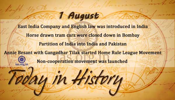
The East India Company and the English law was introduced in India for the first time. It was set up as it was directed by the Court of Judicature.

1774

On this day in 1774, dissenting British minister Joseph Priestly, author of Observations on Civil Liberty and the Nature and Justice of the War with America, discovered oxygen.

1846

Dwarkanath Tagore, a Hindu philanthropist, died in London.

1889

Kamala Nehru, wife of Pandit Jawaharlal Nehru, great revolutionary, freedom fighter and social worker, was born.

1905

Horse drawn tram cars were closed down in Bombay. This service was started on May 9, 1874 with 20 tram cars and 200 horses. The very first day of its run, the number of passengers carried was 451 and the amount earned was Rs. 85/- on the last day it had 1360 horses and carried 71,947 passengers and earned Rs.4,260/.

1914

First World War erupted in Europe

1916

Mrs. Annie Besant in cooperation with Bal Gangadhar Tilak started the Home Rule League Movement with Dadabhai Naoroji as its President.

1920

Bipin Chandra Pal opposed to the Non Co-operation Movement and retired from politics, but movement was approved by Congress.

1920

Under the leadership of Gandhi, the non-cooperation movement was launched against Lord Chelmsford. “Firmness in truth,” was his strategy of non cooperation and non-violence against India’s Christian British rulers. Later, he resolved to wear only ‘dhoti’ to preserve homespun cotton and simplicity, followed with grassroots agitation. This began with renunciation of honorary titles like ‘Sir’ given by the British. Thereafter, it was followed by the boycott of legislatures, elections and other Government works. Foreign clothes were burnt and Khadi became a symbol of freedom. The movement was a great success despite firing and arrests. By the end of 1921, all important national leaders, except Gandhi, were in jail, along with 3000 others. However, in February 1922, at Chaurichaura, Uttar Pradesh, violence erupted and Gandhi called off the movement.

1920

Bal Gangadhar Tilak, British-Indian Hindu leader, died at Bombay.

1920

Kirloskar, monthly magzine, was published.

1920

Gandhiji addressed letter to Viceroy surrendering “Kaisar-E-Hind” Medal, “Zulu War” Medal and “Boer War” Medal and launched the All India Non-Violent Non-Coperation Movement.

1939

Bombay began Prohibition, first since U.S. law was repealed.

1947

Partition of India into India and Pakistan. Power transferred. Lord Mountbatten became Governor General of India and Muhammed Ali Jinnah, Governor General of Pakistan.

1953

All Private Airlines were nationalised by establishing of All Airlines India International.

1953

Bombay Government decided to abolish ”jagirs” in merged areas.

1957

National Book Trust inaugurated.

1958

Ramon Magsaysay Award for community leadership was given to Acharya Bhave.

1962

Establishment of Maharashtra State Industrial Development Corporation.

1963

Soviets offer India arms to block China.

1966

Himachal Pradesh Krishi Vishvavidyalaya (HPKV) was established at Palampur under the aegis of Punjab Agricultural University, Ludhiana, to cater to the need of hilly areas of erstwhile Punjab.

1970

Bhopal University was established.

1971

A severe flood of the Red River in North Vietnam killed an estimated 100,000 people on this day in 1971. This remarkable flood was one of the century’s most serious weather events.

1975

The United States, the Soviet Union, Canada and every European nation (except Albania) signed the Helsinki Final Act on the last day of the Conference on Security and Cooperation in Europe (CSCE). The act was intended to revive the sagging spirit of detente between the Soviet Union and the United States and its allies.

1986

Amnesty scheme for evaders of taxes announced.

1994

The Railway passenger insurance scheme came into force.

2000

The Lok Sabha adopted Uttar Pradesh State Reorganisation Bill paving the way for the creation of Uttaranchal the 27th State.

2007

On this day in 2007, Citibank opened China’s first drive-through automated teller machine (ATM) at the Upper East Side Central Plaza in Beijing.

Related Articles:

Today in History – 30 July

Today in History – 29 July

Today in History – 28 July

Today in History – 27 July

Radial Equations and Quantum Numbers: Unraveling Atomic Structure

0
radial equations quantum numbers

Table of Contents

  1. Introduction
  2. Central Potentials and Radial Schrödinger Equation
  3. Separation of Variables in Spherical Coordinates
  4. Angular Momentum and the Centrifugal Term
  5. Redefining the Radial Equation
  6. Effective Potential and Physical Interpretation
  7. Principal Quantum Number \( n \)
  8. Orbital Angular Momentum Quantum Number \( \ell \)
  9. Radial Nodes and Quantum Number Relationships
  10. Solving the Radial Equation for Hydrogen
  11. Radial Wavefunctions and Laguerre Polynomials
  12. Bohr Radius and Atomic Length Scales
  13. Radial Probability Density
  14. Quantum Numbers and Degeneracy
  15. Extensions to Multi-Electron Atoms
  16. Conclusion

1. Introduction

In atomic quantum mechanics, understanding how the electron behaves within a central potential is key to predicting its energy levels and spatial distribution. The radial equation, derived from the 3D Schrödinger equation, contains essential physics and introduces important quantum numbers that govern atomic structure.


2. Central Potentials and Radial Schrödinger Equation

A central potential depends only on the distance from the origin:

\[
V(\vec{r}) = V(r)
\]

This symmetry allows the use of spherical coordinates \((r, \theta, \phi)\), leading to separable solutions and well-defined angular momentum properties.


3. Separation of Variables in Spherical Coordinates

Assume a total wavefunction:

\[
\psi(r, \theta, \phi) = R(r) Y(\theta, \phi)
\]

Substituting into the time-independent Schrödinger equation and separating variables yields:

  • An angular equation, solved by spherical harmonics \( Y_\ell^m(\theta, \phi) \)
  • A radial equation, which governs the energy and radial probability

4. Angular Momentum and the Centrifugal Term

From the angular solution, we get:

\[
\hat{L}^2 Y_\ell^m = \hbar^2 \ell(\ell+1) Y_\ell^m
\]

This leads to a term in the radial equation:

\[
\frac{\ell(\ell+1)\hbar^2}{2\mu r^2}
\]

Called the centrifugal barrier, it prevents low-\( \ell \) states from collapsing at the origin and shapes the effective potential.


5. Redefining the Radial Equation

Define a new function \( u(r) = r R(r) \). The radial equation becomes:

\[
\frac{d^2 u}{dr^2} + \left[ \frac{2\mu}{\hbar^2}(E – V(r)) – \frac{\ell(\ell+1)}{r^2} \right] u(r) = 0
\]

This is a second-order differential equation whose solutions provide the allowed radial wavefunctions and energy levels.


6. Effective Potential and Physical Interpretation

Rewriting the radial equation:

\[
\frac{d^2 u}{dr^2} + \frac{2\mu}{\hbar^2} \left[E – V_{\text{eff}}(r) \right] u(r) = 0
\]

Where:

\[
V_{\text{eff}}(r) = V(r) + \frac{\hbar^2 \ell(\ell+1)}{2\mu r^2}
\]

  • The second term acts like a repulsive force
  • Influences the turning points and radial confinement

7. Principal Quantum Number \( n \)

The principal quantum number \( n \) labels energy levels:

\[
n = 1, 2, 3, \dots
\]

It arises from boundary conditions ensuring normalizable and finite solutions. In hydrogen-like atoms:

\[
E_n = -\frac{\mu e^4}{2(4\pi\varepsilon_0)^2 \hbar^2 n^2}
\]


8. Orbital Angular Momentum Quantum Number \( \ell \)

The quantum number \( \ell \) arises from solving the angular equation:

  • Determines the shape of the orbital
  • Allowed values: \( \ell = 0, 1, 2, \dots, n-1 \)

It also appears in the centrifugal term, shaping the radial solution.


9. Radial Nodes and Quantum Number Relationships

The number of radial nodes \( n_r \) (zero crossings in \( R(r) \)) is:

\[
n_r = n – \ell – 1
\]

Thus:

  • Ground state (\( n = 1, \ell = 0 \)): 0 nodes
  • Higher \( n \): more nodes, more oscillatory behavior

10. Solving the Radial Equation for Hydrogen

For hydrogen’s Coulomb potential:

\[
V(r) = -\frac{e^2}{4\pi\varepsilon_0 r}
\]

The radial solutions involve associated Laguerre polynomials:

\[
R_{n\ell}(r) = \rho^\ell e^{-\rho/2} L_{n – \ell – 1}^{2\ell + 1}(\rho), \quad \rho = \frac{2r}{n a_0}
\]

Where \( a_0 \) is the Bohr radius.


11. Radial Wavefunctions and Laguerre Polynomials

Radial functions are:

\[
R_{n\ell}(r) = N_{n\ell} \left( \frac{r}{a_0} \right)^\ell e^{-r/(na_0)} L_{n-\ell-1}^{2\ell+1} \left( \frac{2r}{na_0} \right)
\]

These are orthogonal and form a complete basis for bound states.


12. Bohr Radius and Atomic Length Scales

The Bohr radius is:

\[
a_0 = \frac{4\pi \varepsilon_0 \hbar^2}{\mu e^2}
\]

It defines the natural length scale of hydrogenic orbitals.

Typical orbital sizes increase with \( n \), as \( \langle r \rangle \sim n^2 a_0 \).


13. Radial Probability Density

The radial probability density is:

\[
P(r) = |R(r)|^2 r^2
\]

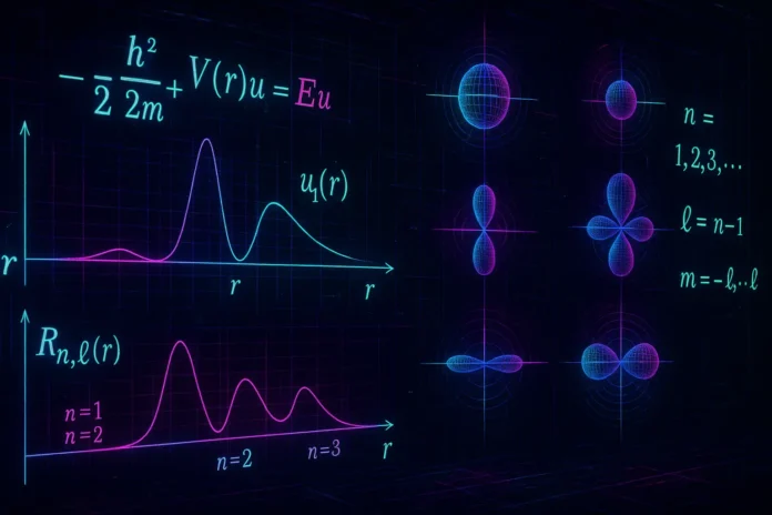
Gives the likelihood of finding the electron at a distance \( r \). Plots of \( P(r) \) show peaks and nodes, visualizing electron shell structure.


14. Quantum Numbers and Degeneracy

Each energy level \( n \) has a degeneracy of:

\[
g_n = n^2 = \sum_{\ell=0}^{n-1} (2\ell + 1)
\]

This reflects the number of allowed \( \ell \) and \( m \) values per \( n \).


15. Extensions to Multi-Electron Atoms

While hydrogen allows exact solutions, in multi-electron atoms:

  • The radial equation is modified by electron shielding
  • \( n \) and \( \ell \) remain, but energies depend on screened nuclear charge
  • Leads to fine structure splitting and shell structures

16. Conclusion

The radial equation lies at the heart of quantum atomic theory. It introduces key quantum numbers that define the structure, energy, and behavior of atomic orbitals. Understanding how radial functions and quantum numbers interplay provides a deeper insight into electron configuration, spectroscopy, and the periodic table.


.

Today in History – 30 July

1
today in history 30 july

today in history 30 july

1622

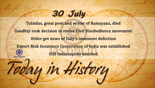
Tulsidas, devotee of God Rama Saint, great poet and writer of Ramayana, died.

1886

Dr. S.Muthulakshmi Reddi, first women M.A.L.A.S, was born.

1933

Gandhiji informed the Government of Bombay of his decision to march from Ahmedabad to Ras with 33 followers to revive Civil Disobedience movement.

1945

On this day in 1945, the USS Indianapolis was torpedoed by a Japanese submarine and sank within minutes in shark-infested waters. Only 317 of the 1,196 men on board survived. However, the Indianapolis had already completed its major mission: the delivery of key components of the atomic bomb that would be dropped a week later at Hiroshima to Tinian Island in the South Pacific.

1947

The part of Kashmir, North West Frontier Provience (NWFP), was swallowed up by Pakistan. The formality of raising the flag was done in November.

1957

Export Risk Insurance Corporation of India was established through which exporting materials were insured.

1960

Gangadhar Balkrishna Deshpande, great freedom fighter, leader and ‘Lion of Karnataka’, died. He was a loyal Congress leader.

1965

On this day in 1965, President Lyndon B. Johnson signed Medicare, a health insurance program for elderly Americans, into law. At the bill-signing ceremony, which took place at the Truman Library in Independence, Missouri, former President Harry S. Truman was enrolled as Medicare’s first beneficiary and received the first Medicare card. Johnson wanted to recognize Truman, who, in 1945, had become the first president to propose national health insurance, an initiative that was opposed at the time by Congress.

1971

A mid-air collision between a Boeing 727 and a fighter jet in Japan killed 162 people on this day in 1971. The military plane was flying without radar.

1975

Thirty-five nations, called together by the United States and the Soviet Union, began a summit meeting in Helsinki, Finland, to discuss some pressing international issues. The meeting temporarily revived the spirit of detente between the United States and Russia.

1987

India says it will revive the ‘Agni‘ IRBM programe.

Related Articles:

Today in History – 29 July

Today in History – 28 July

Today in History – 27 July

Today in History – 26 July

Hydrogen Atom in 3D: Quantum Structure of the Simplest Atom

0
hydrogen atom 3d

Table of Contents

  1. Introduction
  2. Importance of the Hydrogen Atom
  3. Classical vs Quantum Models
  4. The Coulomb Potential and Central Force Problem
  5. Schrödinger Equation in 3D Spherical Coordinates
  6. Separation of Variables
  7. Radial and Angular Parts of the Wavefunction
  8. Angular Solutions: Spherical Harmonics
  9. Radial Equation and Effective Potential
  10. Quantization of Energy Levels
  11. Principal, Orbital, and Magnetic Quantum Numbers
  12. Radial Wavefunctions and Their Nodes
  13. Electron Orbitals and Probability Densities
  14. Degeneracy and Symmetries
  15. Fine Structure and Spin-Orbit Coupling (Preview)
  16. Real-World Applications and Spectroscopy
  17. Conclusion

1. Introduction

The hydrogen atom, consisting of a single proton and electron, serves as the foundation of atomic physics and quantum mechanics. Its study yields exact solutions to the quantum mechanical problem of a charged particle in a Coulomb potential and sets the stage for understanding more complex atoms and molecules.


2. Importance of the Hydrogen Atom

The hydrogen atom is the simplest bound quantum system. Its analytical solution:

  • Validates quantum theory
  • Predicts atomic spectra
  • Helps define quantum numbers and orbitals
  • Introduces tools like angular momentum, spherical harmonics, and radial equations

3. Classical vs Quantum Models

Classical View:

  • Electron orbits nucleus in circular or elliptical path (Bohr model)
  • Discrete orbits postulated without quantum basis

Quantum View:

  • Electron described by wavefunction
  • Energy levels and orbital shapes arise from solving Schrödinger equation

4. The Coulomb Potential and Central Force Problem

In atomic units, the electrostatic potential energy is:

\[
V(r) = -\frac{e^2}{4\pi\varepsilon_0 r}
\]

This spherically symmetric potential makes it a central force problem, ideal for spherical coordinates.


5. Schrödinger Equation in 3D Spherical Coordinates

The time-independent Schrödinger equation:

\[
-\frac{\hbar^2}{2\mu} \nabla^2 \psi(\vec{r}) + V(r)\psi(\vec{r}) = E\psi(\vec{r})
\]

Where:

  • \( \mu \): reduced mass of electron-proton system
  • \( V(r) \): Coulomb potential

In spherical coordinates \((r, \theta, \phi)\), \( \nabla^2 \) becomes:

\[
\nabla^2 = \frac{1}{r^2} \frac{\partial}{\partial r} \left( r^2 \frac{\partial}{\partial r} \right)
\frac{1}{r^2 \sin\theta} \frac{\partial}{\partial \theta} \left( \sin\theta \frac{\partial}{\partial \theta} \right)
\frac{1}{r^2 \sin^2\theta} \frac{\partial^2}{\partial \phi^2}
\]


6. Separation of Variables

Assume solution:

\[
\psi(r, \theta, \phi) = R(r) Y(\theta, \phi)
\]

Insert into Schrödinger equation ⇒ separates into radial and angular parts.


7. Radial and Angular Parts of the Wavefunction

The equation separates into:

Angular Equation:

\[
\hat{L}^2 Y(\theta, \phi) = \hbar^2 \ell(\ell+1) Y(\theta, \phi)
\]

Radial Equation:

\[
\frac{d^2u}{dr^2} + \left[ \frac{2\mu}{\hbar^2} \left(E + \frac{e^2}{4\pi\varepsilon_0 r} \right) – \frac{\ell(\ell + 1)}{r^2} \right] u(r) = 0
\]

Where \( u(r) = r R(r) \) and \( \ell \): orbital angular momentum quantum number.


8. Angular Solutions: Spherical Harmonics

The angular part \( Y_\ell^m(\theta, \phi) \) are spherical harmonics, solutions of:

\[
\hat{L}z Y\ell^m = \hbar m Y_\ell^m, \quad \hat{L}^2 Y_\ell^m = \hbar^2 \ell(\ell+1) Y_\ell^m
\]

With:

  • \( \ell = 0, 1, 2, \dots \)
  • \( m = -\ell, \dots, \ell \)

These define the shapes and orientations of orbitals.


9. Radial Equation and Effective Potential

The radial equation contains an effective potential:

\[
V_{\text{eff}}(r) = -\frac{e^2}{4\pi\varepsilon_0 r} + \frac{\hbar^2 \ell(\ell + 1)}{2\mu r^2}
\]

The second term represents the centrifugal barrier due to angular momentum.


10. Quantization of Energy Levels

Solving the radial equation yields discrete energy levels:

\[
E_n = -\frac{\mu e^4}{2(4\pi\varepsilon_0)^2 \hbar^2 n^2}, \quad n = 1, 2, 3, \dots
\]

These depend only on the principal quantum number \( n \). This degeneracy reflects the high symmetry of the Coulomb potential.


11. Principal, Orbital, and Magnetic Quantum Numbers

  • \( n \): Principal quantum number, \( n \ge 1 \)
  • \( \ell \): Orbital quantum number, \( 0 \le \ell \le n-1 \)
  • \( m \): Magnetic quantum number, \( -\ell \le m \le \ell \)

Each state is labeled \( |n, \ell, m\rangle \).


12. Radial Wavefunctions and Their Nodes

Radial functions are:

\[
R_{n\ell}(r) = \rho^\ell e^{-\rho/2} L_{n-\ell-1}^{2\ell+1}(\rho), \quad \rho = \frac{2r}{na_0}
\]

Where \( L_k^m \) are associated Laguerre polynomials, and \( a_0 \) is the Bohr radius.

  • \( n – \ell – 1 \): number of radial nodes

13. Electron Orbitals and Probability Densities

The electron orbitals (e.g., 1s, 2p, 3d) are visual representations of \( |\psi(r, \theta, \phi)|^2 \).

  • Shape dictated by angular part \( Y_\ell^m \)
  • Size and radial structure by \( R_{n\ell}(r) \)
  • Probability densities are used in atomic imaging and chemistry

14. Degeneracy and Symmetries

Each energy level \( E_n \) has a degeneracy:

\[
g_n = n^2 = \sum_{\ell=0}^{n-1} (2\ell + 1)
\]

Reflecting spherical symmetry and conservation of angular momentum.


15. Fine Structure and Spin-Orbit Coupling (Preview)

Real hydrogen energy levels split slightly due to:

  • Relativistic corrections
  • Spin-orbit coupling
  • Quantum electrodynamic effects (Lamb shift)

These refinements are explained by Dirac theory and QED.


16. Real-World Applications and Spectroscopy

Hydrogen’s spectral lines (Lyman, Balmer series) match energy differences:

\[
\Delta E = E_n – E_{n’}
\]

Explains:

  • Astronomical spectra
  • Atomic clocks
  • Quantum chemistry foundations

17. Conclusion

The 3D hydrogen atom is a landmark success of quantum theory. Its analytical solution explains atomic spectra, defines quantum numbers, and reveals orbital structures. Mastery of this system is essential for advanced quantum mechanics, spectroscopy, chemistry, and quantum computing.


.