Table of Contents

1. Introduction
2. What Is Probability?
3. Sample Spaces and Events
4. Axioms of Probability
5. Conditional Probability
6. Bayes’ Theorem
7. Independent and Dependent Events
8. Random Variables: Discrete and Continuous
9. Probability Distributions
10. Expectation and Variance
11. Common Discrete Distributions
12. Common Continuous Distributions
13. Law of Large Numbers
14. Central Limit Theorem
15. Applications in Science and Engineering
16. Conclusion

---

1. Introduction

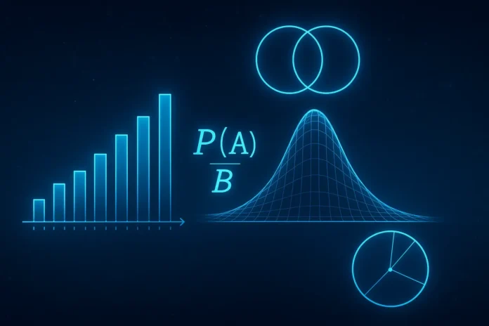
Probability theory provides a rigorous mathematical framework to model uncertainty and randomness. It plays a central role in physics, computer science, statistics, and engineering, allowing us to describe systems where outcomes are not deterministic.

---

2. What Is Probability?

Probability measures the likelihood of a given event occurring, ranging between 0 (impossible) and 1 (certain). In practice, it is used to model uncertain outcomes in experiments, physical systems, and information processes.

---

3. Sample Spaces and Events

• Sample space \( \Omega \): the set of all possible outcomes
• Event: a subset of the sample space

Example:

• Tossing a coin: \( \Omega = \{\text{Heads}, \text{Tails}\} \)
• Rolling a die: \( \Omega = \{1, 2, 3, 4, 5, 6\} \)

---

4. Axioms of Probability

1. Non-negativity: \( P(A) \ge 0 \)
2. Normalization: \( P(\Omega) = 1 \)
3. Additivity: For disjoint events \( A \cap B = \emptyset \),
   \[
   P(A \cup B) = P(A) + P(B)
   \]

---

5. Conditional Probability

The probability of \( A \) given \( B \):

\[
P(A | B) = \frac{P(A \cap B)}{P(B)}, \quad \text{if } P(B) > 0
\]

Describes dependent probabilities based on partial information.

---

6. Bayes’ Theorem

A fundamental result relating conditional probabilities:

\[
P(A | B) = \frac{P(B | A) P(A)}{P(B)}
\]

Used in:

• Statistical inference
• Machine learning
• Decision theory

---

7. Independent and Dependent Events

Events \( A \) and \( B \) are independent if:

\[
P(A \cap B) = P(A) P(B)
\]

Otherwise, they are dependent — knowing one affects the probability of the other.

---

8. Random Variables: Discrete and Continuous

A random variable is a function assigning numbers to outcomes in a sample space.

• Discrete: countable outcomes (e.g., coin toss)
• Continuous: uncountably many outcomes (e.g., height, time)

---

9. Probability Distributions

• Discrete: probability mass function (PMF): \( P(X = x) \)
• Continuous: probability density function (PDF): \( f(x) \)

Cumulative distribution function (CDF):

\[
F(x) = P(X \le x)
\]

---

10. Expectation and Variance

• Expected value (mean):

\[
\mathbb{E}[X] = \sum x_i P(x_i) \quad \text{(discrete)}, \quad \mathbb{E}[X] = \int x f(x) dx \quad \text{(continuous)}
\]

• Variance:

\[
\text{Var}(X) = \mathbb{E}[(X – \mu)^2] = \mathbb{E}[X^2] – (\mathbb{E}[X])^2
\]

---

11. Common Discrete Distributions

• Bernoulli: two outcomes (0 or 1)
• Binomial: \( n \) independent Bernoulli trials
• Geometric: trials until first success
• Poisson: rare events per unit time or space

---

12. Common Continuous Distributions

• Uniform: equal probability over interval
• Normal (Gaussian):
  \[
  f(x) = \frac{1}{\sqrt{2\pi\sigma^2}} e^{-(x – \mu)^2 / 2\sigma^2}
  \]
• Exponential: time between events in Poisson process
• Gamma, Beta, Chi-square: advanced distributions in physics/statistics

---

13. Law of Large Numbers

As the number of trials increases:

\[
\frac{1}{n} \sum_{i=1}^n X_i \to \mathbb{E}[X] \quad \text{(in probability)}
\]

Describes long-run stability of averages.

---

14. Central Limit Theorem

If \( X_1, …, X_n \) are i.i.d. with mean \( \mu \) and variance \( \sigma^2 \), then:

\[
\frac{\sum X_i – n\mu}{\sqrt{n}\sigma} \to \mathcal{N}(0,1)
\]

Important result justifying normal approximations in statistics.

---

15. Applications in Science and Engineering

• Quantum mechanics: probabilistic nature of measurement
• Thermodynamics: statistical interpretation of entropy
• Signal processing: noise modeling
• Finance: option pricing and risk analysis
• Machine learning: probabilistic models and inference

---

16. Conclusion

Probability theory equips us with tools to reason about randomness, uncertainty, and complex systems. From simple experiments to stochastic processes in physics and data science, understanding these fundamentals is crucial for advanced theoretical and practical applications.

---

Table of Contents

1. Introduction
2. What Are Partial Differential Equations?
3. Order, Linearity, and Classification
4. First-Order PDEs
5. Method of Characteristics
6. Second-Order Linear PDEs
7. Classification: Elliptic, Parabolic, Hyperbolic
8. Canonical Forms and Transformation of Variables
9. The Heat Equation
10. The Wave Equation
11. Laplace’s and Poisson’s Equations
12. Boundary and Initial Conditions
13. Separation of Variables
14. Fourier Series Solutions
15. Green’s Functions and Integral Methods
16. Numerical Methods for PDEs
17. Applications in Physics and Engineering
18. Conclusion

---

1. Introduction

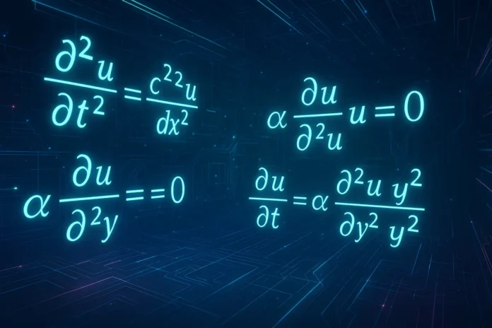
Partial Differential Equations (PDEs) involve multivariable functions and their partial derivatives. They are the natural language of physics — describing phenomena from heat and sound propagation to electromagnetism and quantum mechanics.

---

2. What Are Partial Differential Equations?

A PDE relates a function \( u(x_1, x_2, …, x_n) \) to its partial derivatives:

\[
F\left(x_i, u, \frac{\partial u}{\partial x_i}, \frac{\partial^2 u}{\partial x_i \partial x_j}, \dots \right) = 0
\]

They generalize ODEs to functions of several variables.

---

3. Order, Linearity, and Classification

• Order: Highest derivative present
• Linear: Linear in \( u \) and all derivatives
• Quasilinear: Linear in highest derivatives only
• Nonlinear: Nonlinear in derivatives or the function

Example:

• Linear: \( u_{xx} + u_{yy} = 0 \)
• Nonlinear: \( u_t + u u_x = 0 \)

---

4. First-Order PDEs

General form:

\[
a(x, y, u) \frac{\partial u}{\partial x} + b(x, y, u) \frac{\partial u}{\partial y} = c(x, y, u)
\]

Methods:

• Method of characteristics
• Change of variables

---

5. Method of Characteristics

Converts PDE into a system of ODEs:

\[
\frac{dx}{a} = \frac{dy}{b} = \frac{du}{c}
\]

Solves for characteristic curves along which the PDE reduces to an ODE.

---

6. Second-Order Linear PDEs

General form in two variables:

\[
A u_{xx} + B u_{xy} + C u_{yy} + D u_x + E u_y + Fu = G
\]

The type of PDE depends on the discriminant \( B^2 – 4AC \):

• Elliptic: \( B^2 – 4AC < 0 \)
• Parabolic: \( B^2 – 4AC = 0 \)
• Hyperbolic: \( B^2 – 4AC > 0 \)

---

7. Classification: Elliptic, Parabolic, Hyperbolic

• Elliptic: steady-state (e.g., Laplace’s equation)
• Parabolic: diffusion-type (e.g., heat equation)
• Hyperbolic: wave-like (e.g., wave equation)

---

8. Canonical Forms and Transformation of Variables

PDEs can often be simplified by change of variables:

• Elliptic → \( u_{\xi\xi} + u_{\eta\eta} = 0 \)
• Hyperbolic → \( u_{\xi\eta} = 0 \)

This reduces complexity and aids analytical solutions.

---

9. The Heat Equation

Describes temperature evolution:

\[
\frac{\partial u}{\partial t} = \alpha \frac{\partial^2 u}{\partial x^2}
\]

Parabolic; models diffusion of heat, particles, etc.

---

10. The Wave Equation

Describes wave propagation:

\[
\frac{\partial^2 u}{\partial t^2} = c^2 \frac{\partial^2 u}{\partial x^2}
\]

Hyperbolic; solution involves traveling waves and d’Alembert’s formula.

---

11. Laplace’s and Poisson’s Equations

• Laplace: \( \nabla^2 u = 0 \)
• Poisson: \( \nabla^2 u = f(x, y) \)

Elliptic; describe electrostatics, fluid flow, and potential theory.

---

12. Boundary and Initial Conditions

Well-posed problems require:

• Initial condition for time evolution
• Boundary conditions (Dirichlet, Neumann, or Robin) on spatial domain

---

13. Separation of Variables

Assumes:

\[
u(x, t) = X(x)T(t)
\]

Reduces PDE to ODEs in separate variables, solvable via eigenfunction expansions.

---

14. Fourier Series Solutions

Periodic boundary conditions allow expansion in sine and cosine:

\[
u(x, t) = \sum_{n=1}^\infty A_n(t) \sin\left(\frac{n\pi x}{L}\right)
\]

Used to solve heat and wave equations on bounded domains.

---

15. Green’s Functions and Integral Methods

A Green’s function \( G(x, x’) \) solves:

\[
L G(x, x’) = \delta(x – x’)
\]

Allows us to write the solution as an integral:

\[
u(x) = \int G(x, x’) f(x’) dx’
\]

Powerful for inhomogeneous boundary value problems.

---

16. Numerical Methods for PDEs

When analytical solutions are not possible:

• Finite difference methods
• Finite element methods
• Spectral methods

Used in simulations across physics and engineering.

---

17. Applications in Physics and Engineering

• Electromagnetism: Maxwell’s equations
• Quantum mechanics: Schrödinger equation
• Fluid dynamics: Navier–Stokes equations
• Acoustics: Helmholtz equation
• Heat transfer: heat equation

---

18. Conclusion

Partial Differential Equations are central to modeling and solving multidimensional, dynamic physical problems. Understanding their classification, solutions, and applications is critical for modern physics, engineering, and applied mathematics.

From electrostatics to quantum fields, PDEs provide the mathematical lens through which we study and simulate the world.

---

Table of Contents

1. Introduction
2. What Is an Ordinary Differential Equation?
3. Order and Linearity
4. First-Order ODEs
5. Separable Equations
6. Linear First-Order Equations
7. Exact Equations and Integrating Factors
8. Second-Order Linear ODEs
9. Homogeneous and Inhomogeneous Equations
10. Characteristic Equation and Solution Space
11. Method of Undetermined Coefficients
12. Variation of Parameters
13. Systems of First-Order ODEs
14. Qualitative Analysis and Phase Space
15. Applications in Physics and Engineering
16. Conclusion

---

1. Introduction

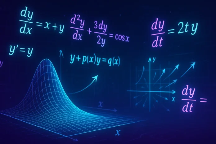
Ordinary Differential Equations (ODEs) describe how a quantity evolves with respect to one independent variable — typically time or space. They are essential in modeling motion, growth, decay, oscillations, and fields in physics, biology, economics, and engineering.

---

2. What Is an Ordinary Differential Equation?

An ODE involves a function and its derivatives with respect to a single variable:

\[
F\left(x, y, \frac{dy}{dx}, \frac{d^2y}{dx^2}, \dots \right) = 0
\]

---

3. Order and Linearity

• Order: highest derivative present
• Linearity: linear if the dependent variable and its derivatives appear to the first power and are not multiplied together

Example:

• Linear: \( y” + 3y’ + 2y = 0 \)
• Nonlinear: \( y” + y(y’) = x \)

---

4. First-Order ODEs

General form:

\[
\frac{dy}{dx} = f(x, y)
\]

Can be solved via:

• Separation of variables
• Integrating factors
• Substitutions

---

5. Separable Equations

\[
\frac{dy}{dx} = g(x)h(y)
\Rightarrow \frac{1}{h(y)}dy = g(x)dx
\]

Integrate both sides to obtain the solution.

---

6. Linear First-Order Equations

Standard form:

\[
\frac{dy}{dx} + P(x)y = Q(x)
\]

Use integrating factor:

\[
\mu(x) = e^{\int P(x) dx}
\Rightarrow y(x) = \frac{1}{\mu(x)} \int \mu(x) Q(x) dx
\]

---

7. Exact Equations and Integrating Factors

An equation \( M(x, y)dx + N(x, y)dy = 0 \) is exact if:

\[
\frac{\partial M}{\partial y} = \frac{\partial N}{\partial x}
\]

Then there exists a potential function \( \psi(x, y) \) such that \( d\psi = 0 \). Otherwise, use an integrating factor to make it exact.

---

8. Second-Order Linear ODEs

General form:

\[
a(x)y” + b(x)y’ + c(x)y = f(x)
\]

If \( f(x) = 0 \), the equation is homogeneous; otherwise, non-homogeneous.

---

9. Homogeneous and Inhomogeneous Equations

• Homogeneous: solutions form a vector space
• Inhomogeneous: general solution is the sum of the homogeneous solution and a particular solution

---

10. Characteristic Equation and Solution Space

For constant coefficients:

\[
y” + ay’ + by = 0 \Rightarrow r^2 + ar + b = 0
\]

Roots \( r_1, r_2 \) determine the solution:

• Real and distinct → \( y = C_1 e^{r_1 x} + C_2 e^{r_2 x} \)
• Real and equal → \( y = (C_1 + C_2 x)e^{r x} \)
• Complex → \( y = e^{\alpha x}(C_1 \cos \beta x + C_2 \sin \beta x) \)

---

11. Method of Undetermined Coefficients

Used for inhomogeneous equations with \( f(x) \) like:

• \( e^{ax} \), \( \sin bx \), \( \cos bx \), polynomials

Guess a solution form, substitute, and solve for constants.

---

12. Variation of Parameters

General solution for inhomogeneous equation:

\[
y = y_h + y_p
\]

Where \( y_h \) is the homogeneous solution, and \( y_p \) is:

\[
y_p = u_1(x)y_1(x) + u_2(x)y_2(x)
\]

Found via integration using Wronskian.

---

13. Systems of First-Order ODEs

Written as:

\[
\frac{d\vec{y}}{dx} = A(x)\vec{y} + \vec{b}(x)
\]

Can be solved via matrix exponentials, diagonalization, or numerical methods.

---

14. Qualitative Analysis and Phase Space

• Equilibrium points
• Stability analysis using Jacobian
• Phase portraits visualize trajectories in state space

Used in nonlinear dynamics and control theory.

---

15. Applications in Physics and Engineering

• Harmonic oscillator: \( m\ddot{x} + kx = 0 \)
• RC circuits: \( V = IR + \frac{1}{C} \int I dt \)
• Radioactive decay: \( \frac{dN}{dt} = -\lambda N \)
• Newton’s laws: \( F = ma \Rightarrow \frac{d^2x}{dt^2} = \frac{F}{m} \)

---

16. Conclusion

Ordinary differential equations are the mathematical backbone of time-evolution problems in science and engineering. From simple decay to complex oscillatory systems, ODEs model the continuous change of systems in precise, analyzable form.

Understanding their classification, solution methods, and qualitative behavior is essential for anyone studying mathematical or physical sciences.

---