

Home Blog Page 302

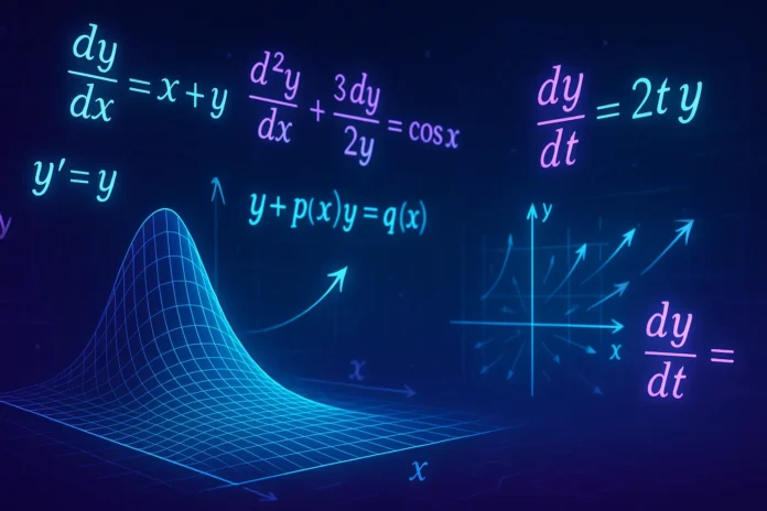
Ordinary Differential Equations (ODEs): Foundations, Methods, and Applications

0
Differential Equations

Table of Contents

  1. Introduction
  2. What Is an Ordinary Differential Equation?
  3. Order and Linearity
  4. First-Order ODEs
  5. Separable Equations
  6. Linear First-Order Equations
  7. Exact Equations and Integrating Factors
  8. Second-Order Linear ODEs
  9. Homogeneous and Inhomogeneous Equations
  10. Characteristic Equation and Solution Space
  11. Method of Undetermined Coefficients
  12. Variation of Parameters
  13. Systems of First-Order ODEs
  14. Qualitative Analysis and Phase Space
  15. Applications in Physics and Engineering
  16. Conclusion

1. Introduction

Ordinary Differential Equations (ODEs) describe how a quantity evolves with respect to one independent variable — typically time or space. They are essential in modeling motion, growth, decay, oscillations, and fields in physics, biology, economics, and engineering.


2. What Is an Ordinary Differential Equation?

An ODE involves a function and its derivatives with respect to a single variable:

\[
F\left(x, y, \frac{dy}{dx}, \frac{d^2y}{dx^2}, \dots \right) = 0
\]


3. Order and Linearity

  • Order: highest derivative present
  • Linearity: linear if the dependent variable and its derivatives appear to the first power and are not multiplied together

Example:

  • Linear: \( y” + 3y’ + 2y = 0 \)
  • Nonlinear: \( y” + y(y’) = x \)

4. First-Order ODEs

General form:

\[
\frac{dy}{dx} = f(x, y)
\]

Can be solved via:

  • Separation of variables
  • Integrating factors
  • Substitutions

5. Separable Equations

\[
\frac{dy}{dx} = g(x)h(y)
\Rightarrow \frac{1}{h(y)}dy = g(x)dx
\]

Integrate both sides to obtain the solution.


6. Linear First-Order Equations

Standard form:

\[
\frac{dy}{dx} + P(x)y = Q(x)
\]

Use integrating factor:

\[
\mu(x) = e^{\int P(x) dx}
\Rightarrow y(x) = \frac{1}{\mu(x)} \int \mu(x) Q(x) dx
\]


7. Exact Equations and Integrating Factors

An equation \( M(x, y)dx + N(x, y)dy = 0 \) is exact if:

\[
\frac{\partial M}{\partial y} = \frac{\partial N}{\partial x}
\]

Then there exists a potential function \( \psi(x, y) \) such that \( d\psi = 0 \). Otherwise, use an integrating factor to make it exact.


8. Second-Order Linear ODEs

General form:

\[
a(x)y” + b(x)y’ + c(x)y = f(x)
\]

If \( f(x) = 0 \), the equation is homogeneous; otherwise, non-homogeneous.


9. Homogeneous and Inhomogeneous Equations

  • Homogeneous: solutions form a vector space
  • Inhomogeneous: general solution is the sum of the homogeneous solution and a particular solution

10. Characteristic Equation and Solution Space

For constant coefficients:

\[
y” + ay’ + by = 0 \Rightarrow r^2 + ar + b = 0
\]

Roots \( r_1, r_2 \) determine the solution:

  • Real and distinct → \( y = C_1 e^{r_1 x} + C_2 e^{r_2 x} \)
  • Real and equal → \( y = (C_1 + C_2 x)e^{r x} \)
  • Complex → \( y = e^{\alpha x}(C_1 \cos \beta x + C_2 \sin \beta x) \)

11. Method of Undetermined Coefficients

Used for inhomogeneous equations with \( f(x) \) like:

  • \( e^{ax} \), \( \sin bx \), \( \cos bx \), polynomials

Guess a solution form, substitute, and solve for constants.


12. Variation of Parameters

General solution for inhomogeneous equation:

\[
y = y_h + y_p
\]

Where \( y_h \) is the homogeneous solution, and \( y_p \) is:

\[
y_p = u_1(x)y_1(x) + u_2(x)y_2(x)
\]

Found via integration using Wronskian.


13. Systems of First-Order ODEs

Written as:

\[
\frac{d\vec{y}}{dx} = A(x)\vec{y} + \vec{b}(x)
\]

Can be solved via matrix exponentials, diagonalization, or numerical methods.


14. Qualitative Analysis and Phase Space

  • Equilibrium points
  • Stability analysis using Jacobian
  • Phase portraits visualize trajectories in state space

Used in nonlinear dynamics and control theory.


15. Applications in Physics and Engineering

  • Harmonic oscillator: \( m\ddot{x} + kx = 0 \)
  • RC circuits: \( V = IR + \frac{1}{C} \int I dt \)
  • Radioactive decay: \( \frac{dN}{dt} = -\lambda N \)
  • Newton’s laws: \( F = ma \Rightarrow \frac{d^2x}{dt^2} = \frac{F}{m} \)

16. Conclusion

Ordinary differential equations are the mathematical backbone of time-evolution problems in science and engineering. From simple decay to complex oscillatory systems, ODEs model the continuous change of systems in precise, analyzable form.

Understanding their classification, solution methods, and qualitative behavior is essential for anyone studying mathematical or physical sciences.


.

Today in History – 11 June

0
today in history 11 june

today in history 11 june

1776

On this day in 1776, the Continental Congress selected Thomas Jefferson of Virginia, John Adams of Massachusetts, Benjamin Franklin of Pennsylvania, Roger Sherman of Connecticut and Robert R. Livingston of New York to draft a declaration of independence.

1880

Jeannette Pickering Rankin, the first woman ever elected to Congress, was born on a ranch near Missoula, Montana Territory. Rankin was a social worker in the states of Montana and Washington before joining the women’s suffrage movement in 1910.

1907

Shantilal Jivanlal Gandhi, famous Hindi writer, was born in Mehmadabad, Gujarat .

1931

Purushottam Vishnu Behre, great editor, story and novel writer, was born.

1946

Viceroy interviewed Gandhiji, and mooted proposal of Coalition Government at Centre.

1964

Dr. Jayant Narlikar, great mathematician of India, submitted his thesis to Royal Society of London.

1976

Indira Gandhi and Brezhnev signed the Moscow Declaration of Friendship and Cooperation.

1983

Ghanshyam Das Birla, great freedom fighter, social reformer, pioneer of Indian business, industry, and nationalist, died at London at the age of 89.

1997

I.K. Gujral, PM, asserted that India had not deployed the `Prithvi’ ballistic missile anywhere in the country or on the border.

1997

Jaspal Rana and J. Abhijit in the men’s section and Nisha Millet in the women’s section adjudged best sports persons of the National Games.

1999

India provided incontrovertible tape evidence of Pakistan’s involvement in the Kargil sector. The Indian army killed 23 intruders in the Batalik and Dras sectors but lost 15 of its men.

Related Articles:

Today in History – 10 June

Today in History – 9 June

Today in History – 8 June

Today in History – 7 June

Delta Function and Distributions: Foundations for Generalized Function Theory

0
Delta Function and Distributions

Table of Contents

  1. Introduction
  2. Motivation: Beyond Classical Functions
  3. The Dirac Delta Function
  4. Properties of the Delta Function
  5. Representations and Approximations
  6. Delta Function in Multiple Dimensions
  7. Derivatives of the Delta Function
  8. Heaviside Step Function and Relation to Delta
  9. Distributions and Test Functions
  10. Action of Distributions on Test Functions
  11. Schwartz Distributions and Linear Functionals
  12. Fourier Transform of the Delta Function
  13. Delta Function in Physics
  14. Applications in Quantum Mechanics and Electrodynamics
  15. Conclusion

1. Introduction

The Dirac delta function and the theory of distributions extend classical calculus to include objects like impulses, point charges, and discontinuities. While not functions in the traditional sense, they are indispensable in physics and engineering for modeling idealized phenomena.


2. Motivation: Beyond Classical Functions

In many physical situations, we want to describe:

  • A point mass or point charge
  • An instantaneous force
  • A perfect impulse at a single point in time or space

Classical functions cannot handle these cases. Distributions (or generalized functions) allow us to rigorously define and manipulate such concepts.


3. The Dirac Delta Function

The Dirac delta function \( \delta(x) \) is defined via its action:

\[
\int_{-\infty}^{\infty} \delta(x) f(x) dx = f(0)
\]

More generally:

\[
\int_{-\infty}^{\infty} \delta(x – a) f(x) dx = f(a)
\]

It “picks out” the value of the function at the point \( x = a \).


4. Properties of the Delta Function

  • Localization: \( \delta(x – a) = 0 \) for \( x \ne a \)
  • Sifting property:
    \[
    \int_{-\infty}^{\infty} \delta(x – a) f(x) dx = f(a)
    \]
  • Evenness: \( \delta(-x) = \delta(x) \)
  • Scaling:
    \[
    \delta(ax) = \frac{1}{|a|} \delta(x)
    \]
  • Change of variable:
    \[
    \delta(g(x)) = \sum_i \frac{\delta(x – x_i)}{|g'(x_i)|}
    \]
    where \( x_i \) are the simple roots of \( g(x) \)

5. Representations and Approximations

The delta function can be approximated by a sequence of functions:

  • Gaussian:
    \[
    \delta_\epsilon(x) = \frac{1}{\epsilon \sqrt{\pi}} e^{-x^2/\epsilon^2}
    \]
  • Lorentzian:
    \[
    \delta_\epsilon(x) = \frac{1}{\pi} \frac{\epsilon}{x^2 + \epsilon^2}
    \]
  • Rectangular:
    \[
    \delta_\epsilon(x) =
    \begin{cases}
    \frac{1}{2\epsilon}, & |x| < \epsilon \
    0, & \text{otherwise}
    \end{cases}
    \]

As \( \epsilon \to 0 \), all tend weakly to \( \delta(x) \).


6. Delta Function in Multiple Dimensions

In \( \mathbb{R}^n \):

\[
\int_{\mathbb{R}^n} \delta(\vec{x} – \vec{a}) f(\vec{x}) \, d^n x = f(\vec{a})
\]

Used in electrostatics, quantum field theory, and Green’s functions.


7. Derivatives of the Delta Function

Distributions can be differentiated:

\[
\int \delta'(x – a) f(x) dx = -f'(a)
\]

This extends to higher derivatives and plays a role in solving differential equations with singular sources.


8. Heaviside Step Function and Relation to Delta

The Heaviside function \( \theta(x) \) is defined as:

\[
\theta(x) =
\begin{cases}
0, & x < 0 \
1, & x \ge 0
\end{cases}
\]

Its derivative (in the distributional sense) is the delta function:

\[
\frac{d}{dx} \theta(x) = \delta(x)
\]


9. Distributions and Test Functions

A distribution is a linear functional \( T \) acting on a test function \( \phi(x) \in \mathcal{D}(\mathbb{R}) \), the space of smooth functions with compact support:

\[
T(\phi) = \int_{-\infty}^{\infty} t(x) \phi(x) dx
\]

Where \( t(x) \) may be singular.


10. Action of Distributions on Test Functions

All calculations are done in terms of pairing:

\[
\langle \delta(x – a), \phi(x) \rangle = \phi(a)
\]

\[
\langle \delta^{(n)}(x – a), \phi(x) \rangle = (-1)^n \phi^{(n)}(a)
\]

This avoids direct evaluation of singularities.


11. Schwartz Distributions and Linear Functionals

In the Schwartz distribution framework:

  • Distributions generalize functions
  • Differentiation becomes continuous
  • Singular behaviors like jumps and spikes are manageable

This is used in quantum field theory and generalized Green’s functions.


12. Fourier Transform of the Delta Function

\[
\mathcal{F}\{\delta(x)\} = 1
\]

\[
\mathcal{F}\{1\} = 2\pi \delta(\omega)
\]

These identities are fundamental in signal analysis and quantum mechanics.


13. Delta Function in Physics

  • Point charge: \( \rho(\vec{r}) = q \delta(\vec{r} – \vec{r}_0) \)
  • Initial conditions: \( f(t) = \delta(t – t_0) \)
  • Green’s functions: \( L G(x, x’) = \delta(x – x’) \)
  • Scattering theory: transition amplitudes involve delta functions

14. Applications in Quantum Mechanics and Electrodynamics

  • Wavefunctions: normalized via delta
    \[
    \langle x | x’ \rangle = \delta(x – x’)
    \]
  • Commutation relations: involve delta
  • Green’s functions: fundamental solutions to field equations

15. Conclusion

The Dirac delta function and the theory of distributions revolutionized the mathematical handling of singularities and idealizations in physics. From modeling point charges to solving field equations, these generalized objects provide clarity, precision, and powerful tools in theoretical and applied sciences.

Understanding them is essential for any serious student of physics or applied mathematics.


.

Today in History – 10 June

0
today in history 10 june

today in history 10 june

1246

Allauddin Masood Shah, Sultan of Dehli, was thrown off the throne.

1752

On this day in 1752, Benjamin Franklin flied a kite during a thunderstorm and collected a charge in a Leyden jar when the kite got struck by lightning, enabled him to demonstrate the electrical nature of lightning. Franklin became interested in electricity in the mid-1740s, a time when much was still unknown on the topic, and spent almost a decade conducting electrical experiments. He coined a number of terms used today, including battery, conductor and electrician. He also invented the lightning rod, used to protect buildings and ships.

1833

Azad Muhammad Jussain, Urdu poet and educationalist, was born.

1888

Balraj Bhalla, revolutionary, was born.

1890

Sunday introduced as a weekly holiday.

1891

Gandhiji was called to the Bar.

1900

Jayantnath Chaudhary, former General of Indian Army General, was born.

1942

77 Mountain Brigade was raised at Sagar, Madhya Pradesh.

1946

Gandhiji refused to enthuse over allied victory as it was not a “victory of truth”.

1955

Prakash Padukone, internationally famous Badminton player, was born.

1957

Bhai Vir Singh, great Punjabi poet, novelist, social reformer, musician, humanitarian and Padma Bhushan awardee, died

1966

MIG aeroplanes were designed at Nashik.

1980

In South Africa, the African National Congress (ANC) made public a statement by Nelson Mandela, the long imprisoned leader of the anti-apartheid movement. The message, smuggled out of Robben Island prison under great risk, read, “UNITE! MOBILISE! FIGHT ON! BETWEEN THE ANVIL OF UNITED MASS ACTION AND THE HAMMER OF THE ARMED STRUGGLE WE SHALL CRUSH APARTHEID!”

1991

On this day in 1991 at Clark Air Base in the Philippines, 14,500 personnel were evacuated in anticipation of the eruption of Mount Pinatubo. Over the next several days, the eruptions killed hundreds of people and sent tons of ash and sulfur dioxide into the atmosphere.

1997

Three Indians – Kumaramangalam Birla, Ratan Tata and Dhirubhai Ambani – figure in the list of Asia’s top 100 super rich.

Related Articles:

Today in History – 9 June

Today in History – 8 June

Today in History – 7 June

Today in History- 6 June

Fourier Series and Transforms: Analyzing Signals in Time and Frequency

0
Fourier Series and Transforms

Table of Contents

  1. Introduction
  2. Motivation: Why Fourier Analysis?
  3. Fourier Series: Periodic Function Decomposition
  4. Orthogonality of Trigonometric Functions
  5. Fourier Coefficients
  6. Convergence of Fourier Series
  7. Even and Odd Functions
  8. Complex Exponential Form of Fourier Series
  9. The Fourier Transform
  10. Properties of the Fourier Transform
  11. Inverse Fourier Transform
  12. The Dirac Delta and Fourier Theory
  13. Discrete Fourier Transform (DFT) and FFT
  14. Applications in Physics and Engineering
  15. Conclusion

1. Introduction

Fourier series and transforms allow us to represent functions in terms of sinusoids and complex exponentials. This is not only mathematically elegant, but also practical for solving differential equations, analyzing signals, and understanding physical systems in terms of their frequency content.


2. Motivation: Why Fourier Analysis?

Many physical systems exhibit oscillatory behavior — vibrations, waves, circuits, or signals.

Decomposing a function into a sum (or integral) of simpler, periodic functions helps us:

  • Analyze behavior in the frequency domain
  • Solve partial differential equations
  • Understand resonance, filtering, and spectral content

3. Fourier Series: Periodic Function Decomposition

Let \( f(x) \) be periodic with period \( 2\pi \). Then:

\[
f(x) = \frac{a_0}{2} + \sum_{n=1}^{\infty} \left( a_n \cos(nx) + b_n \sin(nx) \right)
\]

This expresses \( f(x) \) as a weighted sum of harmonics.


4. Orthogonality of Trigonometric Functions

The key to Fourier decomposition is orthogonality:

\[
\int_{-\pi}^{\pi} \cos(nx)\cos(mx) dx =
\begin{cases}
0, & n \neq m \
\pi, & n = m \neq 0
\end{cases}
\]

\[
\int_{-\pi}^{\pi} \sin(nx)\cos(mx) dx = 0
\]


5. Fourier Coefficients

The coefficients are computed as:

\[
a_n = \frac{1}{\pi} \int_{-\pi}^{\pi} f(x)\cos(nx) dx, \quad
b_n = \frac{1}{\pi} \int_{-\pi}^{\pi} f(x)\sin(nx) dx
\]

\[
a_0 = \frac{1}{\pi} \int_{-\pi}^{\pi} f(x) dx
\]


6. Convergence of Fourier Series

Fourier series converges:

  • Pointwise for piecewise continuous functions
  • Uniformly if the function is continuous and has a continuous derivative

The Gibbs phenomenon refers to overshoots near discontinuities.


7. Even and Odd Functions

  • For even functions, \( b_n = 0 \)
  • For odd functions, \( a_n = 0 \)

This symmetry simplifies the computation of Fourier series.


8. Complex Exponential Form of Fourier Series

Using Euler’s formula:

\[
f(x) = \sum_{n=-\infty}^{\infty} c_n e^{inx}
\]

Where:

\[
c_n = \frac{1}{2\pi} \int_{-\pi}^{\pi} f(x) e^{-inx} dx
\]

This form is convenient in physics and electrical engineering.


9. The Fourier Transform

For a non-periodic function \( f(t) \), the Fourier transform is:

\[
\mathcal{F}\{f(t)\} = F(\omega) = \int_{-\infty}^{\infty} f(t)e^{-i\omega t} dt
\]

It generalizes Fourier series to arbitrary functions.


10. Properties of the Fourier Transform

  • Linearity: \( \mathcal{F}\{af + bg\} = aF + bG \)
  • Time shift: \( f(t – t_0) \leftrightarrow e^{-i\omega t_0} F(\omega) \)
  • Frequency shift: \( e^{i\omega_0 t}f(t) \leftrightarrow F(\omega – \omega_0) \)
  • Differentiation: \( \frac{d^n f}{dt^n} \leftrightarrow (i\omega)^n F(\omega) \)

11. Inverse Fourier Transform

Recovers \( f(t) \) from \( F(\omega) \):

\[
f(t) = \frac{1}{2\pi} \int_{-\infty}^{\infty} F(\omega) e^{i\omega t} d\omega
\]


12. The Dirac Delta and Fourier Theory

The Dirac delta function \( \delta(t) \) is defined as:

\[
\delta(t) = \frac{1}{2\pi} \int_{-\infty}^{\infty} e^{i\omega t} d\omega
\]

Used to express impulse responses and fundamental identities in transform theory.


13. Discrete Fourier Transform (DFT) and FFT

In computation, we use:

\[
X_k = \sum_{n=0}^{N-1} x_n e^{-2\pi i kn/N}
\]

  • DFT converts discrete data from time to frequency
  • FFT is an efficient algorithm to compute DFT in \( O(N \log N) \) time

Used in signal processing, communications, and image analysis.


14. Applications in Physics and Engineering

  • Signal processing: filters, compression, analysis
  • Quantum mechanics: wavefunctions in momentum space
  • Acoustics: harmonic content of sound
  • Optics: diffraction and interference patterns
  • Heat and wave equations: solution via separation and transform

15. Conclusion

Fourier series and transforms bridge time and frequency domains. They enable a deep understanding of oscillatory phenomena and play a vital role in solving differential equations, analyzing systems, and processing data.

In physics, they reveal symmetry, periodicity, and conserved quantities across a wide spectrum of domains.


.