

Home Blog Page 259

Quantum Vacuum and Casimir Effect

0

Table of Contents

  1. Introduction
  2. Classical Vacuum vs Quantum Vacuum
  3. Zero-Point Energy
  4. Quantization of Fields and Vacuum Energy
  5. Normal Ordering and Renormalization
  6. Physical Meaning of Vacuum Fluctuations
  7. Casimir Effect: Historical Background
  8. Casimir Force Between Parallel Plates
  9. Derivation of Casimir Energy
  10. Regularization Techniques
  11. Role of Boundary Conditions
  12. Experimental Verification of Casimir Effect
  13. Lifshitz Theory and Real Materials
  14. Temperature Corrections and Finite Conductivity
  15. Casimir Effect in Different Geometries
  16. Casimirโ€“Polder Forces
  17. Dynamical Casimir Effect
  18. Casimir Effect in Curved Spacetimes
  19. Casimir Effect and Extra Dimensions
  20. Casimir Energy and Cosmological Constant
  21. Quantum Vacuum in Quantum Field Theory
  22. Vacuum Polarization and Virtual Particles
  23. Casimir Effect in Condensed Matter Systems
  24. Applications and Technological Implications
  25. Conclusion

1. Introduction

The quantum vacuum is not empty space but a seething background of fluctuations due to quantum field theory. One of its most striking observable consequences is the Casimir effect, where vacuum fluctuations induce a measurable force between uncharged, conducting plates.


2. Classical Vacuum vs Quantum Vacuum

In classical physics, the vacuum is defined as the absence of matter and fields. In quantum theory, the vacuum state is the ground state of a field, filled with zero-point energy and virtual particles.


3. Zero-Point Energy

Quantizing a harmonic oscillator yields:

\[
E_n = \hbar \omega \left(n + \frac{1}{2} \right)
\]

Even in the ground state \( n = 0 \), there is nonzero energy:

\[
E_0 = \frac{1}{2} \hbar \omega
\]

This persists in field quantization as an infinite sum over modes.


4. Quantization of Fields and Vacuum Energy

For a scalar field \( \phi \), the vacuum energy density is:

\[
\rho_{\text{vac}} = \frac{1}{2} \sum_{\vec{k}} \hbar \omega_{\vec{k}} \quad \to \quad \infty
\]

This divergence must be regularized and renormalized to extract physical meaning.


5. Normal Ordering and Renormalization

Normal ordering redefines the vacuum energy to zero by subtracting infinities. However, in non-trivial geometries (e.g., boundaries), differences in vacuum energy can be finite and physically observable.


6. Physical Meaning of Vacuum Fluctuations

Vacuum fluctuations lead to:

  • Lamb shift
  • Spontaneous emission
  • Casimir effect

These are evidence that the quantum vacuum has real physical effects, despite being unobservable directly.


7. Casimir Effect: Historical Background

Predicted by Hendrik Casimir in 1948. He considered two perfectly conducting, uncharged plates in vacuum and found an attractive force due to the change in vacuum energy.


8. Casimir Force Between Parallel Plates

Two plates separated by distance \( a \) in vacuum experience a pressure:

\[
F = -\frac{\pi^2 \hbar c}{240 a^4} A
\]

where \( A \) is the area of the plates. The force is:

  • Independent of charge
  • Purely quantum mechanical
  • Inversely proportional to the fourth power of separation

9. Derivation of Casimir Energy

The energy between plates is:

\[
E = \frac{\hbar c \pi^2 A}{720 a^3}
\]

Derived by comparing vacuum energy inside and outside the plates, using mode summation and regularization.


10. Regularization Techniques

To deal with infinities in the mode sums:

  • Zeta function regularization
  • Cut-off methods
  • Dimensional regularization

These extract finite, physical parts of divergent sums.


11. Role of Boundary Conditions

Casimir effect arises from the alteration of vacuum modes due to boundaries. Different boundary conditions (Dirichlet, Neumann, periodic) result in different forces โ€” and even repulsive Casimir effects in certain setups.


12. Experimental Verification of Casimir Effect

First verified experimentally in 1997 by Steve Lamoreaux. Modern experiments use:

  • Microelectromechanical systems (MEMS)
  • Atomic force microscopes
  • Cryogenic setups

Agreement with theory is within a few percent.


13. Lifshitz Theory and Real Materials

Lifshitz extended the Casimir theory to real materials with dielectric properties. It accounts for:

  • Finite conductivity
  • Temperature dependence
  • Material dispersion

The Casimirโ€“Lifshitz formula involves the reflection coefficients of materials.


14. Temperature Corrections and Finite Conductivity

At non-zero temperature \( T \), thermal photons contribute to the Casimir force:

\[
F_T = F_0 + \Delta F_T
\]

Finite conductivity reduces the force due to imperfect reflection at high frequencies.


15. Casimir Effect in Different Geometries

Casimir forces are highly geometry-dependent:

  • Parallel plates: attractive
  • Spheres and cylinders: more complex
  • Cavities and topological boundaries: modify vacuum modes

Casimir repulsion is possible under specific boundary and material conditions.


16. Casimirโ€“Polder Forces

Between atoms and conducting surfaces, vacuum fluctuations induce Casimirโ€“Polder forces. These differ from van der Waals forces by incorporating retardation effects:

\[
F(r) \propto \frac{1}{r^7} \quad (\text{non-retarded}), \quad \frac{1}{r^8} \quad (\text{retarded})
\]


17. Dynamical Casimir Effect

If boundaries move rapidly, virtual photons can become real โ€” leading to photon creation from vacuum. Observed in superconducting circuits and optical cavities.


18. Casimir Effect in Curved Spacetimes

In curved spacetimes (e.g., around black holes or expanding universes), the vacuum energy depends on curvature and topology, leading to gravitational Casimir-like effects.


19. Casimir Effect and Extra Dimensions

In theories with compactified extra dimensions (e.g., Kaluza-Klein, string theory), Casimir energy can stabilize extra dimensions or contribute to cosmological dynamics.


20. Casimir Energy and Cosmological Constant

The observed cosmological constant is many orders of magnitude smaller than naive estimates from vacuum energy โ€” the cosmological constant problem. Casimir energies in different vacua highlight this discrepancy.


21. Quantum Vacuum in Quantum Field Theory

In QFT, the vacuum is a rich structure:

  • Ground state of the Hamiltonian
  • Carries fluctuations and correlations
  • Source of particle creation

22. Vacuum Polarization and Virtual Particles

Vacuum fluctuations cause polarization of the vacuum, modifying propagators and effective charges โ€” central to QED phenomena like:

  • Running of the fine-structure constant
  • Lamb shift

23. Casimir Effect in Condensed Matter Systems

Analogues of Casimir effect arise in:

  • Superfluid helium
  • Liquid crystals
  • Boseโ€“Einstein condensates
  • Graphene and 2D materials

24. Applications and Technological Implications

Casimir forces impact:

  • Nanoelectromechanical systems (NEMS)
  • Stiction in microdevices
  • Quantum sensors
  • Precision measurement experiments

25. Conclusion

The quantum vacuum is a fundamental concept that reshapes our understanding of emptiness and energy. The Casimir effect provides direct evidence of vacuum fluctuations and their physical consequences. It bridges quantum field theory, electromagnetism, condensed matter, and cosmology โ€” demonstrating that even nothingness has structure and power.

.

Effective Field Theories

0

Table of Contents

  1. Introduction
  2. Motivation and Basic Idea
  3. Hierarchies of Scales in Physics
  4. Separation of Scales and Decoupling
  5. Classical vs Quantum Field Theory Perspectives
  6. Integrating Out Heavy Degrees of Freedom
  7. Matching and Running Couplings
  8. Wilsonian Effective Action
  9. The Role of Renormalization
  10. Power Counting and Expansion Schemes
  11. Examples of Effective Field Theories
  12. Fermi Theory of Weak Interactions
  13. Chiral Perturbation Theory
  14. Heavy Quark Effective Theory (HQET)
  15. Soft-Collinear Effective Theory (SCET)
  16. Nonrelativistic QED and QCD
  17. Effective Field Theory of Gravity
  18. Quantum Gravity as an EFT
  19. EFTs in Cosmology and Inflation
  20. EFTs in Condensed Matter Physics
  21. Limitations and Validity of EFTs
  22. Matching UV Completions
  23. Symmetries and Anomalies in EFTs
  24. Experimental Tests and Precision Physics
  25. Conclusion

1. Introduction

Effective Field Theories (EFTs) provide a powerful framework to describe physical systems at a given energy scale, without requiring a complete knowledge of high-energy (ultraviolet or UV) physics. They exploit the hierarchy of scales in nature and encode low-energy phenomena in terms of local operators organized by their relevance.


2. Motivation and Basic Idea

In real-world physics, we rarely have access to the complete theory at all scales. Instead, EFTs allow us to describe physics at low energies by:

  • Retaining only light degrees of freedom
  • Encapsulating high-energy effects via higher-dimension operators

3. Hierarchies of Scales in Physics

Natural systems have multiple scales:

  • Atomic physics: \( E \ll m_e \)
  • Nuclear physics: \( E \ll m_W \)
  • Gravity: \( E \ll M_{\text{Planck}} \)

EFTs enable modeling of such systems by focusing only on the relevant scales.


4. Separation of Scales and Decoupling

Appelquistโ€“Carazzone decoupling theorem:
Heavy particles decouple at low energies. Their effects appear as suppressed corrections:

\[
\mathcal{L}{\text{eff}} = \mathcal{L}{\text{light}} + \frac{1}{\Lambda} \mathcal{O}_5 + \frac{1}{\Lambda^2} \mathcal{O}_6 + \cdots
\]

where \( \Lambda \) is the heavy scale and \( \mathcal{O}_i \) are local operators.


5. Classical vs Quantum Field Theory Perspectives

At the classical level, one might simply omit heavy fields. But at the quantum level, loop corrections from heavy particles remain and must be captured systematically through matching procedures.


6. Integrating Out Heavy Degrees of Freedom

Given a full theory with both light (\( \phi \)) and heavy (\( \Phi \)) fields, the path integral becomes:

\[
\int \mathcal{D}\phi \mathcal{D}\Phi \, e^{i S[\phi, \Phi]} \to \int \mathcal{D}\phi \, e^{i S_{\text{eff}}[\phi]}
\]

This results in nonlocal terms, which can be expanded in a derivative (momentum) expansion.


7. Matching and Running Couplings

Matching ensures the EFT reproduces the full theory’s observables at a given scale. Couplings in the EFT run with scale, governed by the renormalization group equations (RGEs).


8. Wilsonian Effective Action

Kenneth Wilson’s formulation:

  • Integrate out momentum shells \( \Lambda – d\Lambda < p < \Lambda \)
  • Flow of couplings described by RGEs
  • Fixed points characterize universality classes

9. The Role of Renormalization

EFTs are renormalizable in the modern sense:

  • Predictive at any order in expansion
  • Renormalization absorbs loop divergences into redefined coefficients
  • Operators organized by dimension and symmetry

10. Power Counting and Expansion Schemes

Operators in the EFT are ordered by their mass dimension \( d \):

  • \( d = 4 \): marginal (renormalizable)
  • \( d < 4 \): relevant
  • \( d > 4 \): irrelevant

Expansion parameter: \( E / \Lambda \)


11. Examples of Effective Field Theories

EFTs appear across physics:

  • Fermi theory of beta decay
  • Chiral perturbation theory in QCD
  • HQET in heavy quark systems
  • Gravity at low energies

12. Fermi Theory of Weak Interactions

Before the electroweak theory, weak interactions were modeled by a 4-fermion contact term:

\[
\mathcal{L}F = -\frac{G_F}{\sqrt{2}} (\bar{p} \gamma^\mu n)(\bar{e} \gamma\mu \nu_e)
\]

Valid for energies \( E \ll m_W \), derived by integrating out the \( W \)-boson.


13. Chiral Perturbation Theory

Low-energy QCD with pions as Goldstone bosons of broken chiral symmetry:

\[
\mathcal{L}{\chi PT} = \frac{f\pi^2}{4} \text{Tr}(\partial_\mu U^\dagger \partial^\mu U) + \cdots
\]

Expansion in \( p/\Lambda_\chi \), where \( \Lambda_\chi \sim 1 \, \text{GeV} \)


14. Heavy Quark Effective Theory (HQET)

Describes systems with heavy quarks (e.g., charm, bottom):

\[
\mathcal{L}{\text{HQET}} = \bar{h}_v iv \cdot D h_v + \frac{1}{2m_Q} \mathcal{O}{\text{kin}} + \cdots
\]

Exploits symmetries in the heavy mass limit.


15. Soft-Collinear Effective Theory (SCET)

Used for processes involving collimated energetic particles (jets), e.g., in collider physics. Resums logarithms and separates soft/collinear dynamics.


16. Nonrelativistic QED and QCD

EFTs for nonrelativistic bound states:

  • Hydrogen atom
  • Quarkonium

Treat expansions in \( v/c \) and separate Coulombic and radiative contributions.


17. Effective Field Theory of Gravity

General relativity treated as an EFT:

\[
\mathcal{L} = \sqrt{-g} \left( \frac{1}{16\pi G} R + c_1 R^2 + c_2 R_{\mu\nu} R^{\mu\nu} + \cdots \right)
\]

Predictive below \( M_{\text{Planck}} \), useful for quantum corrections to classical GR.


18. Quantum Gravity as an EFT

Despite being non-renormalizable, gravity can be studied as an EFT:

  • Loop corrections are finite and calculable order-by-order
  • Black hole entropy, gravitational waves, and inflation involve EFT methods

19. EFTs in Cosmology and Inflation

EFT of inflation:
\[
\mathcal{L} = -\frac{1}{2} (\partial \phi)^2 – V(\phi) + \frac{1}{\Lambda^4} (\partial \phi)^4 + \cdots
\]

Systematic way to study inflationary perturbations and non-Gaussianities.


20. EFTs in Condensed Matter Physics

Effective theories describe low-energy excitations:

  • Phonons in solids
  • Spin waves in magnets
  • Fermi liquids
  • Superfluidity and superconductivity

21. Limitations and Validity of EFTs

EFTs are valid only below their cutoff scale \( \Lambda \). At energies \( E \sim \Lambda \), the full UV theory must be invoked. EFTs do not determine UV completions โ€” they encode low-energy consequences.


22. Matching UV Completions

Different UV theories can lead to the same EFT at low energies โ€” a manifestation of universality. Matching procedures relate parameters of the EFT to those of the full theory.


23. Symmetries and Anomalies in EFTs

Symmetries restrict allowed operators. Anomalies may be inherited or emerge. Examples include:

  • Chiral anomalies
  • Trace anomalies
  • Gauge anomalies in effective gauge theories

24. Experimental Tests and Precision Physics

EFTs underpin:

  • Precision electroweak tests
  • Higgs coupling studies
  • BSM searches via dimension-6 operators
  • Low-energy neutrino and flavor physics

25. Conclusion

Effective field theories are indispensable tools for modern theoretical and experimental physics. They allow us to model complex systems with unknown high-energy behavior, organize predictions systematically, and make contact with experiment. By respecting symmetry and exploiting scale separation, EFTs bridge fundamental theory and observable phenomena across domains โ€” from nuclear physics and particle interactions to cosmology and gravity.


.

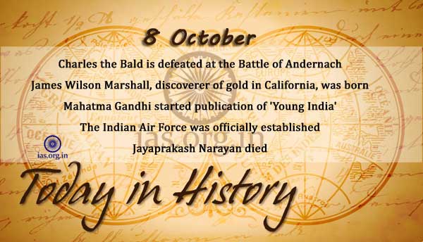
Today in History – 8 October

1
Today in History - 8 October

Today in History - 8 October

876

Charles the Bald is defeated at the Battle of Andernach.

1810

James Wilson Marshall, discoverer of gold in California, was born.

1880

Ernest F E Douwes Dekker, Dutch founder of National India Party, was born.

1900

Maximilian Harden is sentenced to six months in prison for publishing an article critical of the German Kaiser.

1912

First Balkan War begins as Montenegro declares war against the Ottoman Empire.

1919

Mahatma Gandhi started publication of ‘Young India’.

1921

Indian nationalists call a general strike on Prince of Wales’s arrival in Bombay.

1922

Lilian Gatlin becomes the first woman pilot to fly across the United States.

1927

Raaj Kumar, famous Hindi film actor, was born.

1932

The Indian Air Force was officially established, being the date of its formal constitution as India’s first Air Force.

1967

Guerrilla Che Guevara captured in Bolivia.

1978

Jayaprakash Narayan died.

1998

16 policemen are killed when their vehicle is blown up by PWG naxalites on the Basaguda-Jagargunda road in Madhya Pradesh’s Bastar division.

2001

US President George W. Bush establishes the Office of Homeland Security.

Also Read:

Non-Commutative Geometry

0

Table of Contents

  1. Introduction
  2. Motivation and Historical Background
  3. Classical Geometry and Commutativity
  4. Quantum Mechanics and Non-Commuting Observables
  5. From Commutative to Non-Commutative Spaces
  6. Basics of Non-Commutative Algebras
  7. Spectral Triples and the Connes Formalism
  8. Distance in Non-Commutative Geometry
  9. Dirac Operator and the Geometry of the Standard Model
  10. Moyal Plane and Deformation Quantization
  11. Quantum Field Theory on Non-Commutative Spaces
  12. UV/IR Mixing and Renormalization
  13. Gauge Theories in Non-Commutative Geometry
  14. Applications in Matrix Models and String Theory
  15. Emergence from String Theory: D-branes and B-fields
  16. Non-Commutative Spacetime and Quantum Gravity
  17. Planck Scale Physics and Minimal Length
  18. Lorentz Symmetry and Non-Commutativity
  19. Non-Commutative Geometry in Loop Quantum Gravity
  20. C*-Algebras and Operator Theory
  21. Spectral Action Principle
  22. Non-Commutative Cosmology
  23. Experimental Constraints and Physical Realizations
  24. Challenges and Future Directions
  25. Conclusion

1. Introduction

Non-commutative geometry (NCG) generalizes the concepts of geometry and topology to spaces where coordinates do not commute. It provides a powerful framework for describing spacetime at the quantum scale, with deep implications for quantum gravity, high-energy physics, and the foundations of geometry.


2. Motivation and Historical Background

Traditional geometry is based on commuting coordinates:
\[
[x^\mu, x^\nu] = 0
\]
But quantum mechanics and attempts at quantum gravity motivate the study of geometries where:
\[
[x^\mu, x^\nu] = i \theta^{\mu\nu}
\]
This is the central idea of non-commutative geometry.


3. Classical Geometry and Commutativity

In classical differential geometry:

  • Points are elements of a manifold
  • Functions commute under multiplication
  • Geometry is encoded in the algebra of smooth functions \( C^\infty(M) \)

4. Quantum Mechanics and Non-Commuting Observables

Quantum mechanics introduces non-commutativity:
\[
[\hat{x}, \hat{p}] = i\hbar
\]
This suggests that spacetime itself might become non-commutative at small scales, with position coordinates no longer commuting.


5. From Commutative to Non-Commutative Spaces

Alain Connes proposed that geometry can be reformulated algebraically:

  • Commutative algebra โ†” classical space
  • Non-commutative algebra โ†” quantum space

Geometry becomes the study of operator algebras.


6. Basics of Non-Commutative Algebras

A non-commutative algebra \( \mathcal{A} \) is an associative algebra where:
\[
ab \neq ba
\]
Examples include:

  • Matrix algebras
  • Moyal algebra
  • Operator algebras on Hilbert spaces

7. Spectral Triples and the Connes Formalism

A spectral triple \( (\mathcal{A}, \mathcal{H}, D) \) defines a non-commutative geometry:

  • \( \mathcal{A} \): Algebra of coordinates
  • \( \mathcal{H} \): Hilbert space of states
  • \( D \): Dirac operator encoding metric information

This framework generalizes Riemannian geometry to the non-commutative realm.


8. Distance in Non-Commutative Geometry

The Connes distance formula defines the distance between two pure states \( \phi_1, \phi_2 \):

\[
d(\phi_1, \phi_2) = \sup_{a \in \mathcal{A}} \left\{ |\phi_1(a) – \phi_2(a)| \, : \, | [D, a] | \leq 1 \right\}
\]

This replaces the usual geodesic distance.


9. Dirac Operator and the Geometry of the Standard Model

Using a spectral triple, Connes and collaborators reproduced the Standard Model of particle physics coupled to gravity, including:

  • Higgs mechanism
  • Fermion masses
  • Gauge interactions

All emerge from geometric data in non-commutative space.


10. Moyal Plane and Deformation Quantization

One of the simplest non-commutative geometries:
\[
[x^\mu, x^\nu] = i \theta^{\mu\nu}
\]

Functions on this space are multiplied using the Moyal (star) product:
\[
(f \star g)(x) = f(x) \exp\left(\frac{i}{2} \overleftarrow{\partial}\mu \theta^{\mu\nu} \overrightarrow{\partial}\nu \right) g(x)
\]


11. Quantum Field Theory on Non-Commutative Spaces

NCG modifies field theory:

  • Products of fields are replaced by \( \star \)-products
  • Locality is modified
  • Propagators and interactions receive corrections

12. UV/IR Mixing and Renormalization

Non-commutativity can lead to UV/IR mixing: ultraviolet divergences affect infrared behavior. This complicates renormalization and leads to nonlocal effective actions.


13. Gauge Theories in Non-Commutative Geometry

Gauge transformations are modified:
\[
A_\mu \to U \star A_\mu \star U^\dagger + i U \star \partial_\mu U^\dagger
\]

New features:

  • Enforced non-Abelian structure
  • Modified field strengths
  • Seibergโ€“Witten map relates commutative and non-commutative gauge fields

14. Applications in Matrix Models and String Theory

NCG arises naturally in:

  • Matrix models of M-theory
  • IKKT model (Ishibashiโ€“Kawaiโ€“Kitazawaโ€“Tsuchiya)
  • Matrix-valued coordinates describe emergent non-commutative spacetimes

15. Emergence from String Theory: D-branes and B-fields

In string theory, D-branes in the presence of a background B-field develop non-commutative coordinates on their worldvolume:

\[
[x^\mu, x^\nu] = i \theta^{\mu\nu}
\]

This links NCG to open string dynamics.


16. Non-Commutative Spacetime and Quantum Gravity

NCG is a candidate for describing quantum spacetime:

  • Introduces minimal length
  • Prevents localization below Planck scale
  • May resolve singularities in black holes and cosmology

17. Planck Scale Physics and Minimal Length

A common consequence:
\[
\Delta x \gtrsim \ell_P
\]
This sets a limit to resolution and modifies uncertainty relations โ€” connected with generalized uncertainty principles (GUP).


18. Lorentz Symmetry and Non-Commutativity

NCG can break or deform Lorentz invariance. Alternatives like ฮบ-Minkowski spacetime and Doubly Special Relativity attempt to preserve modified symmetry principles.


19. Non-Commutative Geometry in Loop Quantum Gravity

Though LQG uses a different formalism (spin networks), it shares ideas:

  • Quantized areas and volumes
  • Discrete structure of geometry
  • Operator-valued observables

NCG offers a complementary perspective.


20. C*-Algebras and Operator Theory

Non-commutative spaces are modeled via C*-algebras, generalizing the notion of function algebras. These tools support spectral analysis and provide mathematical rigor.


21. Spectral Action Principle

A central proposal in NCG:
\[
S = \text{Tr}\left( f\left( \frac{D}{\Lambda} \right) \right)
\]
where \( f \) is a cutoff function and \( D \) is the Dirac operator. This yields both gravitational and particle physics actions from geometry.


22. Non-Commutative Cosmology

Modifications to spacetime at early times may lead to:

  • Inflationary corrections
  • Resolution of initial singularity
  • Modified Friedmann equations
  • New phenomenology in cosmic microwave background

23. Experimental Constraints and Physical Realizations

Though Planck-scale non-commutativity is hard to test, indirect bounds arise from:

  • High-energy cosmic rays
  • Gamma-ray bursts
  • Collider experiments
  • Quantum optics and interferometry

24. Challenges and Future Directions

Key challenges:

  • Unifying NCG with full quantum gravity
  • Recovering standard physics at low energies
  • Constructing consistent non-commutative QFTs
  • Connecting with observational data

25. Conclusion

Non-commutative geometry transforms our understanding of space and geometry at the quantum scale. It replaces point-based geometry with operator algebras and introduces fundamental discreteness. With deep connections to string theory, matrix models, and the standard model, NCG continues to illuminate the path toward quantum gravity and a more complete theory of spacetime.


.

Today in History – 7 October

0
Today in History 7 October

Today in History 7 October

1586

The Mughal army entered Srinagar where ‘Khutbah’ was being recited in the name of the emperor.

1708

Guru Govind Singh, tenth and the last Sikh Guru, was assassinated.

1737

40 feet waves sink 20,000 small craft & kill 300,000 (Bengal, India).

1914

Begam Akhtar, famous gazal singer, was born.

1919

Mahatma Gandhij started publication of ‘Navjeevan’ newspaper.

1949

East Germany, the German Democratic Republic, is formed.

1950

Mother Teresa, started Missionaries of Charity, in Calcutta.

1952

Chandigarh became the capital of Punjab.

1993

The Supreme Court rejected private management’s plea for 50\% quota in private professional colleges.

1996

Fox News Channel begins broadcasting.

1997

Central government women employees to get 135 days’ maternity leave and men to get 15 days’ paternity leave.

2000

WWF-India bags the first Rajiv Gandhi Wildlife Conservation Award.

Also Read:

Today in History –ย 6 October

Today in History –ย 4 October

Today in History -3 October

Today in History –ย 1 October