
Home Blog Page 299

Tensor Analysis: The Language of Modern Theoretical Physics

0
tenor analysis

Table of Contents

  1. Introduction
  2. What Is a Tensor?
  3. Scalars, Vectors, and Higher-Rank Tensors
  4. Tensor Notation and Index Conventions
  5. Contravariant and Covariant Tensors
  6. The Metric Tensor and Index Raising/Lowering
  7. Tensor Transformation Laws
  8. Symmetry and Antisymmetry in Tensors
  9. Tensor Operations: Addition, Contraction, Outer Products
  10. Covariant Derivatives and the Connection Coefficients
  11. The Riemann Curvature Tensor
  12. Ricci Tensor and Scalar Curvature
  13. Einstein Tensor and Einstein Field Equations
  14. Tensors in Special and General Relativity
  15. Applications in Continuum Mechanics and Electromagnetism
  16. Conclusion

1. Introduction

Tensors are the mathematical backbone of modern physics, providing a coordinate-independent language to express physical laws. Tensor analysis enables the formulation of theories like general relativity, electromagnetism, and fluid dynamics in a geometric and covariant framework.


2. What Is a Tensor?

A tensor is a geometric object that generalizes scalars and vectors, and transforms in a specific way under coordinate transformations.

A tensor of rank \( (r, s) \) has \( r \) contravariant (upper) and \( s \) covariant (lower) indices:

\[
T^{\mu_1 \dots \mu_r}_{\nu_1 \dots \nu_s}
\]


3. Scalars, Vectors, and Higher-Rank Tensors

  • Scalar: rank-0 tensor, invariant under transformations
  • Vector: rank-1 tensor with one upper index \( V^\mu \)
  • Covector (dual vector): rank-1 tensor with one lower index \( V_\mu \)
  • Rank-2 tensor: \( T^{\mu\nu}, T^\mu{}\nu, T{\mu\nu} \), etc.

4. Tensor Notation and Index Conventions

Einstein summation convention: repeated upper and lower indices are summed:

\[
A^\mu B_\mu = \sum_\mu A^\mu B_\mu
\]

Latin indices typically denote spatial dimensions, Greek for spacetime.


5. Contravariant and Covariant Tensors

  • Contravariant: transforms with inverse Jacobian:

\[
V’^\mu = \frac{\partial x’^\mu}{\partial x^\nu} V^\nu
\]

  • Covariant: transforms with Jacobian:
\[ V’\mu = \frac{\partial x^\nu}{\partial x’^\mu} V\nu \]

Mixed tensors combine both types.


6. The Metric Tensor and Index Raising/Lowering

The metric tensor \( g_{\mu\nu} \) maps vectors to covectors and defines inner products:

\[
V_\mu = g_{\mu\nu} V^\nu, \quad V^\mu = g^{\mu\nu} V_\nu
\]

It also defines distances and angles:

\[
ds^2 = g_{\mu\nu} dx^\mu dx^\nu
\]


7. Tensor Transformation Laws

A tensor of type \( (r, s) \) transforms as:

\[ T’^{\mu_1 \dots \mu_r}{\nu_1 \dots \nu_s} = \frac{\partial x’^{\mu_1}}{\partial x^{\alpha_1}} \dots \frac{\partial x’^{\mu_r}}{\partial x^{\alpha_r}} \frac{\partial x^{\beta_1}}{\partial x’^{\nu_1}} \dots \frac{\partial x^{\beta_s}}{\partial x’^{\nu_s}} T^{\alpha_1 \dots \alpha_r}{\beta_1 \dots \beta_s} \]

8. Symmetry and Antisymmetry in Tensors

  • Symmetric: \( T_{\mu\nu} = T_{\nu\mu} \)
  • Antisymmetric: \( T_{\mu\nu} = -T_{\nu\mu} \)

Antisymmetric rank-2 tensors are used to define quantities like the electromagnetic field tensor.


9. Tensor Operations: Addition, Contraction, Outer Products

  • Addition: valid for tensors of the same type
  • Contraction: sum over one upper and one lower index, reduces rank
  • Outer product: combines tensors into higher-rank tensors

10. Covariant Derivatives and the Connection Coefficients

Ordinary derivatives do not preserve tensor character under transformations.

The covariant derivative \( \nabla_\mu \) includes connection coefficients (Christoffel symbols \( \Gamma^\lambda_{\mu\nu} \)):

\[
\nabla_\mu V^\nu = \partial_\mu V^\nu + \Gamma^\nu_{\mu\lambda} V^\lambda
\]


11. The Riemann Curvature Tensor

Measures the noncommutativity of covariant derivatives:

\[ R^\rho{}{\sigma\mu\nu} = \partial\mu \Gamma^\rho_{\nu\sigma} – \partial_\nu \Gamma^\rho_{\mu\sigma} \] \[\Gamma^\rho_{\mu\lambda} \Gamma^\lambda_{\nu\sigma}\] \[\Gamma^\rho_{\nu\lambda} \Gamma^\lambda_{\mu\sigma} \]

Encodes the intrinsic curvature of spacetime.


12. Ricci Tensor and Scalar Curvature

  • Ricci tensor: contraction of Riemann tensor:

\[
R_{\mu\nu} = R^\lambda{}_{\mu\lambda\nu}
\]

  • Ricci scalar: contraction of Ricci tensor with the metric:

\[
R = g^{\mu\nu} R_{\mu\nu}
\]


13. Einstein Tensor and Einstein Field Equations

The Einstein tensor:

\[
G_{\mu\nu} = R_{\mu\nu} – \frac{1}{2} g_{\mu\nu} R
\]

Einsteinโ€™s field equations:

\[
G_{\mu\nu} = \frac{8\pi G}{c^4} T_{\mu\nu}
\]

Relates curvature of spacetime to energy and momentum.


14. Tensors in Special and General Relativity

  • Special relativity: Minkowski metric \( \eta_{\mu\nu} \), 4-vectors
  • General relativity: dynamic spacetime metric \( g_{\mu\nu}(x) \), curvature tensors

Tensors ensure the general covariance of physical laws.


15. Applications in Continuum Mechanics and Electromagnetism

  • Stress-energy tensor: describes energy, momentum, and stress in a field
  • Electromagnetic field tensor:

\[
F_{\mu\nu} = \partial_\mu A_\nu – \partial_\nu A_\mu
\]

Tensors also describe strain, stress, and deformation in solid mechanics.


16. Conclusion

Tensor analysis provides a powerful and consistent language to describe physical laws in any coordinate system. From general relativity to electromagnetism, it allows elegant and coordinate-independent formulations of complex systems.

Mastery of tensors is crucial for modern theoretical physics and applied mathematical modeling.

.

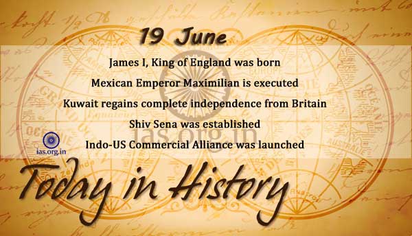
Today in History – 19 June

0
Today in History - 19 June

Today in History - 19 June

240 BC

Eratosthenes estimated the circumference of Earth using two sticks.

1566

James I, King of England (1603-1625), was born.

1747

Nadirshaha passed away.

1867

Mexican Emperor Maximilian was executed.

1934

The National Archives and Records Administration was established.

1949

People of Chandernagar, the French Indian Settlement, decided to merge with the Indian Union.

1961

Kuwait regained complete independence from Britain.

1966

Shiv Sena was established.

1981

APPLE, India’s first experimental geo-stationary telecommunication satellite having experimental communication satellite,was successfully launched by European Ariane, Kourou, French Guiana. This was the first to be stabilized on 3 axes.

1990

NDC approved approach paper to the Eighth Plan.

1995

In an unprecedented move, UP Speaker Dhani Ram Verma adjourned the two-day special session called to prove Mayavati Government’s majority in the House. Later, the House gathers, rejected the sine die adjournment and unanimously elected B.R. Verma (BSP) as new presiding officer to conduct the business of the House.

1995

India and US officially launched Indo-US Commercial Alliance during US Trade Secretary’s visit.

1997

Indian Prime Minister and his Pakistani counterpart Nawaz Sharif, spoke for first time on restored hotline, to reiterate their committment to comprehensive dialogue, including Kashmir.

Also Read:

Today in History –ย 18 June

Today in History –ย 17 June

Today in History –ย 16 June

Today in History –ย 15 June

SU(2), SO(3), and U(1): Key Symmetry Groups in Physics

0
u-2-so-3-u-1

Table of Contents

  1. Introduction
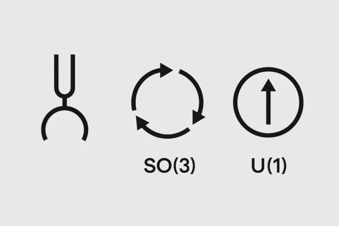
  2. Overview of SU(2), SO(3), and U(1)
  3. U(1): The Simplest Lie Group
  4. U(1) in Physics: Electromagnetism and Phase Invariance
  5. SO(3): The Rotation Group in Three Dimensions
  6. Properties and Structure of SO(3)
  7. Representations of SO(3) and Angular Momentum
  8. SU(2): The Spin Group and Its Significance
  9. SU(2) vs SO(3): Double Cover and Topology
  10. SU(2) Representations and Spin
  11. Pauli Matrices and SU(2) Generators
  12. Embedding SU(2), SO(3), and U(1) in Field Theory
  13. Gauge Symmetries and the Standard Model
  14. Group Manifolds and Global Properties
  15. Conclusion

1. Introduction

SU(2), SO(3), and U(1) are three fundamental Lie groups that appear repeatedly across physics. They describe symmetries in quantum mechanics, gauge theories, and classical systems. Understanding their structure and differences is critical to theoretical physics.


2. Overview of SU(2), SO(3), and U(1)

  • U(1): Group of complex numbers with unit magnitude
  • SO(3): Group of all rotations in 3D space
  • SU(2): Group of 2ร—2 unitary matrices with determinant 1

All are compact, continuous Lie groups, but their topological and algebraic properties differ significantly.


3. U(1): The Simplest Lie Group

U(1) is defined as:

\[
U(1) = \{ e^{i\theta} \mid \theta \in [0, 2\pi) \}
\]

  • Abelian: group elements commute
  • Topologically a circle \( S^1 \)
  • Lie algebra: \( \mathfrak{u}(1) \cong \mathbb{R} \)

4. U(1) in Physics: Electromagnetism and Phase Invariance

  • Governs phase symmetry in quantum mechanics
  • Global U(1): conservation of electric charge (via Noetherโ€™s theorem)
  • Local U(1): leads to electromagnetic gauge theory
  • Appears in the Standard Model as part of \( SU(3) \times SU(2) \times U(1) \)

5. SO(3): The Rotation Group in Three Dimensions

SO(3) consists of real orthogonal \( 3 \times 3 \) matrices with determinant +1:

\[
SO(3) = \{ R \in \mathbb{R}^{3 \times 3} \mid R^T R = I, \ \det R = 1 \}
\]

  • Non-Abelian
  • Describes rigid body rotations in classical mechanics

6. Properties and Structure of SO(3)

  • 3 parameters (e.g., Euler angles)
  • Not simply connected: \( \pi_1(SO(3)) = \mathbb{Z}_2 \)
  • Every rotation corresponds to an axis and angle

7. Representations of SO(3) and Angular Momentum

Quantum angular momentum operators form an \( \mathfrak{so}(3) \) algebra:

\[
[J_i, J_j] = i\hbar \epsilon_{ijk} J_k
\]

  • Representations labeled by integer \( l \): \( l = 0, 1, 2, \dots \)

8. SU(2): The Spin Group and Its Significance

SU(2) consists of \( 2 \times 2 \) unitary matrices with determinant 1:

\[
SU(2) = \left\{
U = \begin{bmatrix} a & b \ -b^* & a^* \end{bmatrix} \mid |a|^2 + |b|^2 = 1
\right\}
\]

  • Non-Abelian
  • Topology: 3-sphere \( S^3 \)
  • Fundamental in spin and weak interactions

9. SU(2) vs SO(3): Double Cover and Topology

  • SU(2) double covers SO(3): \( SU(2)/\mathbb{Z}_2 \cong SO(3) \)
  • SU(2) is simply connected: \( \pi_1(SU(2)) = 0 \)
  • SO(3) is not simply connected: \( \pi_1(SO(3)) = \mathbb{Z}_2 \)

Implication: spin-ยฝ particles (e.g., electrons) described by SU(2), not SO(3)


10. SU(2) Representations and Spin

  • Irreducible representations labeled by half-integers: \( j = 0, \frac{1}{2}, 1, \frac{3}{2}, \dots \)
  • Spin-ยฝ: two-dimensional representation
  • Spin-1: three-dimensional (vector) representation, matches SO(3)

11. Pauli Matrices and SU(2) Generators

Generators of SU(2) are:

\[
T_i = \frac{1}{2} \sigma_i, \quad \text{where } \sigma_i \text{ are the Pauli matrices}
\]

\[
\sigma_1 = \begin{bmatrix} 0 & 1 \ 1 & 0 \end{bmatrix}, \quad
\sigma_2 = \begin{bmatrix} 0 & -i \ i & 0 \end{bmatrix}, \quad
\sigma_3 = \begin{bmatrix} 1 & 0 \ 0 & -1 \end{bmatrix}
\]


12. Embedding SU(2), SO(3), and U(1) in Field Theory

  • SU(2): weak interaction gauge symmetry
  • U(1): electromagnetic gauge symmetry
  • SO(3): spatial symmetry of angular momentum

Combined in electroweak theory via:
\[
SU(2)L \times U(1)_Y \to U(1){\text{EM}}
\]


13. Gauge Symmetries and the Standard Model

  • SU(2) gauge bosons: \( W^+, W^-, W^0 \)
  • U(1) boson: \( B \)
  • Mixing gives photon and \( Z^0 \) boson

Electroweak unification is rooted in the algebra of SU(2) and U(1).


14. Group Manifolds and Global Properties

  • U(1): circle \( S^1 \)
  • SU(2): 3-sphere \( S^3 \)
  • SO(3): 3D projective space \( \mathbb{RP}^3 \)

These properties affect quantization and topological configurations.


15. Conclusion

SU(2), SO(3), and U(1) are foundational symmetry groups in physics. U(1) governs phase invariance and electromagnetism. SO(3) encodes rotational symmetry, while SU(2) is central to spin, angular momentum, and the weak interaction.

Understanding their algebraic and topological properties is essential for any physicist delving into quantum mechanics, particle theory, or gauge symmetries.


.

Today in History – 18 June

0

today in history 18 june

1633

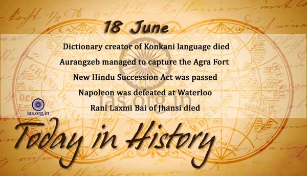
Revairu Diogu, dictionary creator of Konkani language and Jezoet Priest, died.

1658

Aurangzeb managed to capture the Agra Fort and later arrested his father Emperor Shahjahan.

1812

The day after the Senate followed the House of Representatives in voting to declare war against Great Britain, President James Madison signed the declaration into lawโ€“and the War of 1812 began.

1815

At Waterloo in Belgium, Napoleon Bonaparte suffered defeat at the hands of the Duke of Wellington, bringing an end to the Napoleonic era of European history.

1858

Rani Laxmi Bai of Jhansi died while fighting with the British troops in the battlefield near Gwalior.

1887

Dr. Anugrah Narain Singh, freedom fighter, educationist, leader and Minister of India, was born in Poiyavan village, Gaya district, Bihar.

1917

Lachhmansingh Gill, famous politician and former chief minister, was born.

1940

Forward Block Party was established.

1943

British Field Marshal Archibald Wavell becomes Viceroy of India.

1946

First Satyagraha movement was started for Goa liberation from the Portuguese.

1946

Congress Working Committee decided to accept Interim Government scheme.

1956

New Hindu Succession Act was passed.

1966

California’s hippie subculture converged into a mass of long hair, flowers, and rock music this weekend, as 50,000 flowed into the fairgrounds of the Monterey International Pop Festival. The event featured the largest collection of major rock acts ever assembled; thousands of fans had to be turned away from the sold-out concert. Established artists such as the Byrds, Jefferson Airplane, Otis Redding, and the Mamas and the Papas received the expected ovations from the huge audience. But the response was equally enthusiastic for performances by Indian sitar master Ravi Shankar and new talents Janis Joplin, the Who, and Jimi Hendrix, a young man who played the electric guitar like nobody else.

1978

The Karakoram Highway, linking Gilgit in Pakistan-occupied Kashmir with Sinkiang in China, was opened.

1989

India and Pakistan decided to end the five-year-old confrontation in Siachen Glacier area by redeploying their forces.

1983

From Cape Canaveral, Florida, the space shuttle Challenger was launched into space on its second mission. Aboard the shuttle was Dr. Sally Ride, who as a mission specialist who became the first American woman to travel into space.

Related Articles:

Today in History –ย 17 June

Today in History –ย 16 June

Today in History –ย 15 June

Today in History –ย 14 June

Lie Groups and Lie Algebras: Continuous Symmetries in Physics and Geometry

0
lie groups algebras

Table of Contents

  1. Introduction
  2. What Are Lie Groups?
  3. Examples of Lie Groups
  4. Smooth Manifolds and Group Structure
  5. What Is a Lie Algebra?
  6. The Lie Bracket and Commutators
  7. Matrix Lie Groups and Their Algebras
  8. The Exponential Map
  9. Structure Constants and Generators
  10. Representations of Lie Algebras
  11. Cartan Subalgebra and Root Systems
  12. Classification of Simple Lie Algebras
  13. SU(2), SU(3), and SO(n) Algebras
  14. Lie Groups in Physics
  15. Gauge Symmetries and Yang-Mills Theory
  16. Conclusion

1. Introduction

Lie groups and Lie algebras form the mathematical foundation for understanding continuous symmetries. Their theory bridges abstract algebra, differential geometry, and theoretical physics. These structures are essential in classical mechanics, quantum field theory, and the Standard Model of particle physics.


2. What Are Lie Groups?

A Lie group is a group that is also a smooth differentiable manifold, where the group operations (multiplication and inversion) are smooth maps.

Formally, a Lie group \( G \) satisfies:

  • \( G \) is a group
  • \( G \) is a differentiable manifold
  • \( g_1 \cdot g_2 \) and \( g^{-1} \) are smooth maps

3. Examples of Lie Groups

  • \( \mathbb{R}^n \) under addition
  • \( U(1) \): complex numbers of unit magnitude under multiplication
  • \( SU(n) \): special unitary group
  • \( SO(n) \): special orthogonal group (rotations in \( \mathbb{R}^n \))
  • \( GL(n, \mathbb{R}) \): general linear group of invertible \( n \times n \) matrices

4. Smooth Manifolds and Group Structure

Lie groups locally look like Euclidean space. Tangent spaces at each point allow for calculus on groups.

Key property: Lie groups combine local linearity (manifold) with global symmetry (group).


5. What Is a Lie Algebra?

Associated with every Lie group is its Lie algebra, a vector space equipped with a binary operation called the Lie bracket:

\[
[\cdot, \cdot] : \mathfrak{g} \times \mathfrak{g} \to \mathfrak{g}
\]

The Lie algebra \( \mathfrak{g} \) is the tangent space at the identity of the group.


6. The Lie Bracket and Commutators

For matrix Lie groups, the Lie bracket is the commutator:

\[
[X, Y] = XY – YX
\]

Satisfies:

  • Bilinearity
  • Antisymmetry: \( [X, Y] = -[Y, X] \)
  • Jacobi identity:
    \[
    [X, [Y, Z]] + [Y, [Z, X]] + [Z, [X, Y]] = 0
    \]

7. Matrix Lie Groups and Their Algebras

If \( G \subset GL(n, \mathbb{R}) \), then the Lie algebra \( \mathfrak{g} \subset \mathfrak{gl}(n, \mathbb{R}) \) is the space of matrices tangent to \( G \) at the identity.

Example:

  • \( SU(2) \) Lie algebra consists of traceless anti-Hermitian \( 2 \times 2 \) matrices

8. The Exponential Map

Connects the Lie algebra to the group:

\[
\exp: \mathfrak{g} \to G, \quad \exp(X) = \sum_{n=0}^{\infty} \frac{X^n}{n!}
\]

For matrix groups, this is the matrix exponential.

Locally, every element of the group can be written as the exponential of an element of the algebra.


9. Structure Constants and Generators

Let \( \{T_a\} \) be a basis for \( \mathfrak{g} \). Then:

\[
[T_a, T_b] = f^c_{ab} T_c
\]

Where \( f^c_{ab} \) are the structure constants of the algebra.

Generators \( T_a \) represent infinitesimal symmetries.


10. Representations of Lie Algebras

A representation is a map from a Lie algebra to matrices that preserves the bracket:

\[
\rho([X, Y]) = [\rho(X), \rho(Y)]
\]

Irreducible representations are key to understanding particle multiplets, angular momentum, and quantum states.


11. Cartan Subalgebra and Root Systems

  • Cartan subalgebra: maximal commuting set of diagonalizable generators
  • Root system: structure describing how other generators act relative to the Cartan elements

Used in classification of semisimple Lie algebras.


12. Classification of Simple Lie Algebras

Four infinite series:

  • \( A_n = SU(n+1) \)
  • \( B_n = SO(2n+1) \)
  • \( C_n = Sp(2n) \)
  • \( D_n = SO(2n) \)

And five exceptional algebras: \( G_2, F_4, E_6, E_7, E_8 \)


13. SU(2), SU(3), and SO(n) Algebras

  • \( \mathfrak{su}(2) \): spin and angular momentum
  • \( \mathfrak{su}(3) \): QCD color symmetry
  • \( \mathfrak{so}(3) \): rotations in 3D space
  • \( \mathfrak{so}(1,3) \): Lorentz algebra (special relativity)

14. Lie Groups in Physics

  • Symmetry transformations (rotation, translation, boost)
  • Gauge theory: local symmetry leads to gauge bosons
  • Quantum field theory: internal symmetry groups define interactions

15. Gauge Symmetries and Yang-Mills Theory

Gauge fields correspond to Lie algebras:

  • \( SU(3) \): QCD (strong)
  • \( SU(2) \): weak
  • \( U(1) \): electromagnetic

Yangโ€“Mills theory generalizes Maxwellโ€™s equations to non-Abelian gauge groups.


16. Conclusion

Lie groups and Lie algebras provide a deep and powerful language for describing symmetry in mathematics and physics. They underpin quantum field theory, gauge theory, and the Standard Model, and continue to guide modern theoretical research.

Understanding their structure is essential for mastering the modern landscape of high-energy physics and differential geometry.


.