
Home Blog Page 315

Probability Distribution in Quantum Physics: A Deep Dive

0
probaility distribution

Table of Contents

  1. Introduction
  2. Classical vs Quantum Probability
  3. The Wave Function and Probability Amplitude
  4. Born Rule: From Amplitudes to Probabilities
  5. Measurement and Collapse of the Wave Function
  6. Probability Densities in One-Dimensional Systems
  7. Discrete vs Continuous Probability Distributions
  8. Expectation Values and Operators
  9. Probability Currents
  10. Double-Slit Experiment
  11. Quantum Entanglement and Joint Probabilities
  12. Density Matrix Formalism
  13. Path Integrals and Probabilistic Histories
  14. Interpretational Perspectives
  15. Applications
  16. Conclusion

1. Introduction

In classical physics, the future behavior of a system is entirely deterministic if we know its initial conditions. However, in quantum physics, probability is woven into the fabric of reality. Unlike classical randomnessโ€”often stemming from ignoranceโ€”quantum probabilities reflect a fundamental indeterminacy in nature.

This article explores the concept of probability distribution in quantum physics: what it means, how it’s defined, and why itโ€™s central to the interpretation and application of quantum mechanics.


2. Classical vs Quantum Probability

In classical systems, probability often arises from incomplete knowledge. For example, the probability of rolling a six on a die is 1/6โ€‹, assuming fair conditionsโ€”but this reflects our ignorance of the actual physical dynamics at play.

In contrast, quantum probability is inherent. Even with perfect knowledge of the quantum state, outcomes of measurements are fundamentally probabilistic. This difference is not just philosophical but embedded in the mathematics of quantum theory.


3. The Wave Function and Probability Amplitude

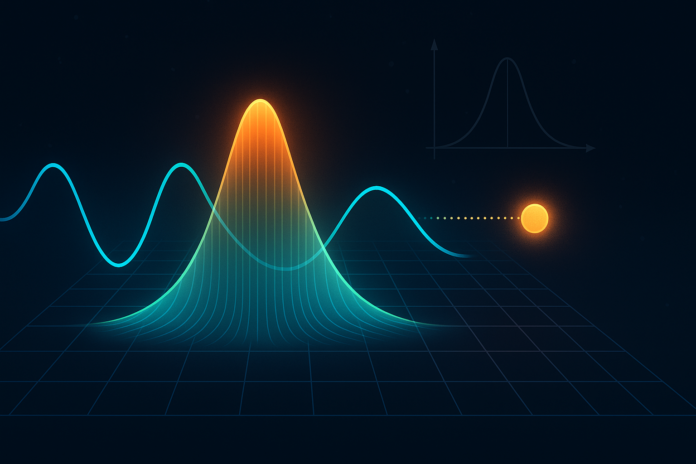
The state of a quantum system is described by a wave function, usually denoted ฯˆ(x,t) for a one-dimensional position-based system. This wave function is a complex-valued function whose modulus squared represents a probability density.

$$ |\psi(x,t)|^2 = \text{Probability density at position } x \text{ and time } t $$

This doesnโ€™t mean the particle is at a particular point until we observe it; it means we can only calculate the likelihood of finding it at that point upon measurement.


4. Born Rule: From Amplitudes to Probabilities

The Born Rule, introduced by Max Born in 1926, formalizes how we extract measurable probabilities from the wave function. If ฯˆ(x,t) is the wave function for a particle, the probability of finding it between positions a and b is:

$$ P(a \leq x \leq b) = \int_a^b |\psi(x,t)|^2 \, dx $$

This rule marks a radical departure from classical physics, emphasizing that the square of a complex amplitude yields a real, observable probability.


5. Measurement and Collapse of the Wave Function

Quantum measurement introduces another probabilistic wrinkle: upon observation, the wave function collapses to a specific eigenstate corresponding to the measurement outcome.

Before measurement, a system exists in a superposition of possible states. Measurement โ€˜choosesโ€™ one of these, seemingly at random, guided by the Born probabilities.

For example, in a position measurement:

  • Before: ฯˆ(x) spread across space
  • After: ฯˆ(x) becomes sharply peaked at the observed value x0x_0x0โ€‹

The probability distribution pre-measurement is replaced by a deterministic post-measurement state.


6. Probability Densities in One-Dimensional Systems

Letโ€™s consider a particle in a one-dimensional infinite potential well (quantum box) of length L. Its normalized wave functions are:

$$ \psi_n(x) = \sqrt{\frac{2}{L}} \sin\left(\frac{n \pi x}{L}\right) $$

The corresponding probability density is:

$$ |\psi_n(x)|^2 = \frac{2}{L} \sin^2\left(\frac{n \pi x}{L}\right) $$

This distribution has nodes and antinodes, unlike classical uniform distribution, and the probability of finding the particle is zero at the walls and specific points inside the well.


7. Discrete vs Continuous Probability Distributions

Quantum systems can have:

  • Discrete probability distributions โ€” e.g., measuring energy levels in a hydrogen atom.
  • Continuous probability distributions โ€” e.g., measuring position or momentum of a free particle.

For discrete states |nโŸฉ, the probability is:

$$ P(n) = |\langle n | \psi \rangle|^2 $$

For continuous variables x:

$$ P(x) = |\psi(x)|^2, \quad \int_{-\infty}^{\infty} P(x) \, dx = 1 $$

This normalization ensures total certainty: the particle must be somewhere.


8. Expectation Values and Operators

Probabilities allow us to compute expectation values, or quantum averages. For an observable represented by operator O^, the expectation value in state ฯˆ is:

$$ \langle \hat{O} \rangle = \int \psi^*(x) \hat{O} \psi(x) \, dx $$

Examples:

  • Position:
$$ \langle x \rangle = \int x |\psi(x)|^2 dx $$
  • Momentum:
$$ \langle p \rangle = \int \psi^*(x)\left(-i\hbar \frac{d}{dx}\right) \psi(x) dx $$

These reflect the center-of-mass or average behavior over many identical measurements.


9. Probability Currents

To track how probability moves through space, we define the probability current density:
Probability current ( j(x,t) ):

$$ j(x,t) = \frac{\hbar}{2mi} \left[ \psi^*(x,t) \frac{\partial \psi(x,t)}{\partial x} – \psi(x,t) \frac{\partial \psi^*(x,t)}{\partial x} \right] $$

Together with the probability density |ฯˆ|2, this satisfies the continuity equation (conservation of probability):

$$ \frac{\partial |\psi|^2}{\partial t} + \frac{\partial j}{\partial x} = 0 $$

This ensures conservation of probability, akin to mass or charge conservation in classical fields.


10. Double-Slit Experiment

The double-slit experiment demonstrates the probabilistic and wave-like nature of quantum particles. When electrons (or photons) pass through two slits, an interference pattern emergesโ€”even when particles go through one at a time.

Each individual detection appears random, but the ensemble distribution aligns perfectly with the square of the total wave amplitudeโ€”reflecting probabilities, not deterministic paths.

Each detection is random, but the probability distribution over many events forms an interference pattern:

$$ P(x) = |\psi_1(x) + \psi_2(x)|^2 $$

where ( \psi_1(x) ) and ( \psi_2(x) ) are amplitudes from each slit.


11. Quantum Entanglement and Joint Probability Distributions

Entangled particles share a joint quantum state. The probability distribution of one particle depends on measurements made on the other, regardless of distanceโ€”a core feature of quantum nonlocality.

For entangled states |ฮจโŸฉ, joint probability P(a,b) for outcomes a and b is:

$$ P(a, b) = |\langle a, b | \Psi \rangle|^2 $$

These probabilitie leads to nonlocal correlations, that violate classical expectations, as shown by Bell inequalities, but remain consistent with quantum formalism.


12. Quantum Probability in Density Matrix Formalism

In mixed states or open systems, we often use the density matrix ฯ where probabilities are extracted via:

$$ P(a) = \text{Tr}(\rho \hat{P}_a) $$

where P^aโ€‹ is the projection operator for outcome aaa. The density matrix generalizes the notion of a pure state to probabilistic ensembles.


13. Path Integrals and Probabilistic Summation

Richard Feynman’s path integral formulation provides a different probabilistic perspective. Instead of wave functions alone, we sum over all possible paths a particle can take from point A to B:

$$ \text{Amplitude} = \sum_{\text{paths}} e^{i S[\text{path}]/\hbar} $$

The interference of these amplitudes determines probabilitiesโ€”an elegant synthesis of quantum and classical perspectives.


14. Quantum Bayesianism (QBism) and Interpretations

Different interpretations of quantum mechanics offer varied views on probability:

  • Copenhagen: Probability reflects intrinsic indeterminacy and wave function collapse.
  • Many Worlds: All outcomes occur in branching universes; probabilities reflect frequency.
  • QBism: Probabilities are Bayesian degrees of belief, personal to the observer.

Each approach reshapes the meaning of the quantum probability distribution while remaining consistent with experimental outcomes.


15. Applications

Probability distributions in quantum mechanics underlie:

  • Quantum algorithms (e.g., Groverโ€™s, Shorโ€™s) which rely on interference and amplitude manipulation.
  • Quantum cryptography, where measurement probability ensures security.
  • Scattering theory, where cross-sections are derived from probability distributions over angular and energy outcomes.
  • Quantum tomography, where states are reconstructed from measured probabilities.

16. Conclusion

Probability distributions in quantum physics are not just tools for making predictionsโ€”they are central to understanding what the theory says about reality itself. The wave function, Born Rule, and collapse postulate form the probabilistic scaffolding upon which the entire structure of quantum mechanics is built.

As research into quantum computing, field theory, and gravity deepens, our grasp of quantum probability continues to evolveโ€”not only mathematically but philosophically, pushing the boundaries of both science and metaphysics.
Today in History – 9 May

0
today in history 9 may

today in history 9 may

1540

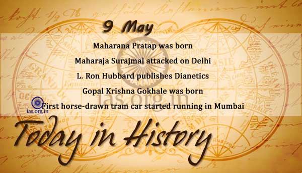
Maharana Pratap, great soldier and a great King , was born.

1753

Maharaja Surajmal attacked on Delhi.

1791

On this day in 1791, Francis Hopkinson, signer of the Declaration of Independence and the first American secular composer, died suddenly of a seizure in Philadelphia, Pennsylvania.

1866

Gopal Krishna Gokhale, freedom fighter and political leader, was born in Kotluk village of Ratnagiri district of Maharashtra.

1874

First horse-drawn tram car started running in Mumbai.

1933

Gandhiji announced suspension of Civil Disobedience Movement for six weeks and called on the Government to withdraw its Ordinances.

1950

On this day in 1950, Lafayette Ronald Hubbard (1911-1986) published Dianetics: The Modern Science of Mental Health. With this book, Hubbard introduced a branch of self-help psychology called Dianetics, which quickly caught fire and, over time, morphed into a belief system boasting millions of subscribers: Scientology.

1959

Karmaveer Bhaurao Patil, founder of Rayat Educational Institute, passed away.

1981

Pandit Sundarlal, great revolutionary and writer of ‘Bharat Mein Angreji Raj’, passed away.

1981

Durga Bai Deshmukh passed away at Hyderabad. She was a social reformer, freedom fighter, planner, administrator, educationist and parliamentarian. She worked for peace, social welfare and for betterment of the downtrodden.

1992

Madhu Sapre, Miss India, is crowned the second runner-up at the Miss Universe beauty pageant.

1992

M.J.Pherwani, National Housing Bank Chairman, resigns following his bank’s involvement in the Security scandal.

1995

Militants set Charar township on fire in the vicinity of the Charar-e-Sherif shrine. More than 1,000 houses burnt.

1995

Two new gas and oil reserves found off the Gujarat and Bombay coast.

1998

Kirit Raval was appointed Solicitor-General of India.

Related Articles:

Today in History – 8 May

Today in History – 5 May

Today in History – 6 May

Today in History  7 May

Quantum Monte Carlo: A Deep Dive into Stochastic Solutions for Quantum Systems

0

Table of Contents

  1. Introduction to Quantum Monte Carlo
  2. Monte Carlo Methods: A Primer
  3. The Quantum Many-Body Problem
  4. Core Quantum Monte Carlo Techniques
    • Variational Monte Carlo (VMC)
    • Diffusion Monte Carlo (DMC)
    • Path Integral Monte Carlo (PIMC)
    • Auxiliary Field Quantum Monte Carlo (AFQMC)
  5. The Fermion Sign Problem
  6. Practical Applications of Quantum Monte Carlo
    • Condensed Matter Physics
    • Quantum Chemistry
    • Nuclear Physics
    • Lattice Quantum Field Theory
  7. Computational Challenges and Strategies
  8. Future of QMC and Emerging Frontiers
  9. Conclusion

1. Introduction to Quantum Monte Carlo

Quantum Monte Carlo (QMC) is a suite of numerical methods designed to solve quantum mechanical problems using stochastic (randomized) algorithms. As quantum systems grow in complexityโ€”such as many-electron atoms, interacting spins on a lattice, or superconducting materialsโ€”exact solutions become computationally infeasible due to exponential growth in the state space. QMC offers a powerful workaround by simulating these systems probabilistically, often producing results with very high accuracy.

While QMC methods vary in formulation and use case, they all share a core strategy: leveraging random sampling to estimate properties of quantum systems. Over time, QMC has become one of the most trusted computational tools in quantum chemistry, condensed matter physics, and quantum field theory.


2. Monte Carlo Methods: A Primer

Before diving into quantum-specific applications, it’s essential to understand Monte Carlo (MC) methods in general. MC methods estimate numerical quantities by using random samples to approximate integrals or solutions to mathematical problems. They’re widely used in finance, physics, statistics, and computer science.

Example:

To estimate the integral of a function f(x) from a to b, MC methods randomly sample points within the interval and average the function values at these points.

Formula:

In the quantum realm, integrals over configuration space, which are often high-dimensional and complex, are similarly approximated using random walks or importance sampling.


3. The Quantum Many-Body Problem

Quantum systems involving multiple particles (electrons, nucleons, etc.) are described by wavefunctions that depend on the coordinates and spins of all particles. For an N-particle system, the wavefunction resides in a 3N-dimensional space (or 4N including spin).

Solving the Schrรถdinger equation directly for these systems is usually intractable:

where H^ is the Hamiltonian operator.

Classical computers struggle with the exponential scaling of quantum state space, which makes QMC’s stochastic approach particularly appealing.


4. Core Quantum Monte Carlo Techniques

4.1 Variational Monte Carlo (VMC)

VMC is the most intuitive and straightforward QMC method. It starts with a trial wavefunction wave function, where r-vector represents the set of particle positions. This wavefunction is parameterized with adjustable variables.

The central idea is to estimate the ground-state energy as:

Using importance sampling, points in configuration space are sampled with a probability distribution probability-distribution, and the local energy local energy equationโ€‹โ€‹ is averaged over the samples.

Key Strengths:

  • Simplicity
  • Easily parallelizable
  • Can be used for optimization

Limitations:

  • Depends on the quality of the trial wavefunction
  • Rarely yields exact ground states

4.2 Diffusion Monte Carlo (DMC)

DMC improves upon VMC by using a projection technique. The wavefunction is evolved in imaginary time to project out the ground state:

This evolution filters out higher-energy states exponentially faster, leaving the ground state in the long-time limit.

The algorithm mimics this evolution via a random walk process combined with branching (weighting and replication of walkers). It is particularly successful in obtaining highly accurate ground-state energies.

Key Strengths:

  • High precision
  • Applicable to both bosons and fermions (with caveats)

Limitations:

  • The fermion sign problem
  • Relies on the fixed-node approximation for fermions
  • Computationally expensive

4.3 Path Integral Monte Carlo (PIMC)

PIMC uses Feynmanโ€™s path integral formulation to model quantum particles as a collection of classical paths in imaginary time. This is particularly effective for simulating finite-temperature systems.

Each quantum particle becomes a polymer-like object, and their interactions are modeled via path integrals. The method is highly accurate for bosonic systems.

Applications:

  • Superfluid helium
  • Quantum dots
  • Bose-Einstein condensates

Limitations:

  • Severely limited by the sign problem for fermions
  • Large memory requirements

4.4 Auxiliary Field Quantum Monte Carlo (AFQMC)

AFQMC transforms two-body interactions into integrals over auxiliary fields using a Hubbard-Stratonovich transformation. The original interacting system becomes a non-interacting system in fluctuating external fields.

This method is used in:

  • Lattice models like the Hubbard model
  • Quantum chemistry for correlated electrons

AFQMC is more flexible and scalable than DMC in some cases, though it also struggles with the sign problem.


5. The Fermion Sign Problem

Perhaps the greatest challenge in QMC for fermionic systems is the sign problem. Because fermionic wavefunctions are antisymmetric, some configurations contribute negatively to the expectation value.

In practice, this leads to cancellations that cause exponential growth in the variance of the simulation:

where N is the number of particles, ฮฒ is inverse temperature, and ฮ”E is the energy gap.

Workarounds:

  • Fixed-node approximation in DMC
  • Constrained path approximation in AFQMC
  • Symmetry restrictions to minimize negative weights

Despite progress, a general solution to the sign problem remains elusive and is an area of active research.


6. Practical Applications of Quantum Monte Carlo

6.1 Condensed Matter Physics

QMC plays a central role in studying electron correlation effects in materials, especially where density functional theory (DFT) fails.

  • Magnetic properties of spin systems
  • High-temperature superconductors
  • Phase transitions in quantum lattices
  • Quantum spin liquids

6.2 Quantum Chemistry

In quantum chemistry, QMC methods offer accuracy that rivals or surpasses coupled-cluster techniques, especially for:

  • Molecular binding energies
  • Reaction barriers
  • Excited states (to a limited extent)

Software packages like QMCPACK and CASINO are designed specifically for molecular simulations using QMC.

6.3 Nuclear Physics

QMC is also used to solve nuclear Hamiltonians with realistic nucleon-nucleon interactions. Techniques like GFMC (Green’s Function Monte Carlo) are adapted for nuclei.

6.4 Lattice Quantum Field Theory

In lattice QCD and other quantum field theories, QMC enables non-perturbative simulations of gauge theories. This has been instrumental in:

  • Computing hadron masses
  • Investigating quark confinement
  • Exploring phase transitions in quantum chromodynamics

7. Computational Challenges and Strategies

Despite its strengths, QMC has a steep computational cost, especially for systems with:

  • Many interacting particles
  • Fermionic statistics
  • High-accuracy demands

Strategies to Mitigate Challenges:

  • Importance sampling: Reduces variance by focusing on high-probability regions.
  • Parallelization: QMC is highly parallelizable and scales well on supercomputers.
  • Machine Learning: Deep neural networks (e.g., FermiNet, PauliNet) are now being integrated to represent wavefunctions more effectively.
  • GPU Acceleration: Hardware acceleration has significantly reduced simulation time.

8. Future of QMC and Emerging Frontiers

QMC continues to evolve in step with advancements in computing and algorithmic innovation.

Emerging Areas:

  • Quantum computing-assisted QMC: Using quantum devices to handle sign-problem-prone parts of the simulation.
  • Neural network wavefunctions: Representing many-body wavefunctions using variational neural networks.
  • Hybrid QMC-DFT methods: Combining the scalability of DFT with the accuracy of QMC.

The field is ripe for interdisciplinary collaborationโ€”spanning physics, computer science, and applied mathematics.


9. Conclusion

Quantum Monte Carlo stands at the frontier of computational quantum mechanics, providing some of the most accurate tools for modeling many-body quantum systems. Despite limitations like the fermion sign problem and high computational demands, QMC methods have proven their worth across physics and chemistry.

As quantum systems become increasingly central to next-generation technologiesโ€”quantum computing, novel materials, and molecular designโ€”QMC will likely grow in relevance, fueled by both algorithmic breakthroughs and advances in computational hardware.

Whether you’re a physicist aiming to understand superconductivity, a chemist optimizing molecular geometries, or a computer scientist building quantum-enhanced algorithms, Quantum Monte Carlo offers a versatile and profound toolkit for probing the quantum world.

Today in History – 8 May

0
today in history 8 may

today in history 8 may

1541

On May 8, 1541, south of present-day Memphis, Tennessee, Spanish conquistador Hernando de Soto reached the Mississippi River, one of the first European explorers to ever do so. After building flatboats, de Soto and his 400 ragged troops crossed the great river under the cover of night, in order to avoid the armed Native Americans who patrolled the river daily in war canoes. From there the conquistadors headed into present-day Arkansas, continuing their fruitless two-year-old search for gold and silver in the American wilderness.

1725

John Lovewell, US Indian fighter, passed away in a battle.

1815

Malaun of Nepal was captured by General David Ochterlony.

1901

British commission claimed famine has taken 1.25 mil. lives since 1899; blames overpopulation.

1906

Prannath Thapar, former General of India, was born.

1910

Tolstoy replies to Gandhi ji that question of Passive Resistance is of greatest importance, not only for India but for humanity.

1930

Gandhi followers mob Bombay to protest his arrest.

1933

Gandhi started hunger strike to protest the British repression of untouchables.

1945

On this day in 1945, both Great Britain and the United States celebrate Victory in Europe Day. Cities in both nations, as well as formerly occupied cities in Western Europe, put out flags and banners, rejoicing in the defeat of the Nazi war machine.

1954

Indian Government decided to integrate Chandranagar in West Bengal which was under the rule of the French.

1959

Dalai Lama will not be allowed to campaign for Tibetan independence in India. India wants to maintain friendly relations with Communist China.

1962

Ravindra Bharti University established in West Bengal.

1963

Centenary of Indian Red Cross was celebrated. Today is birthday of its founder.

1990

A 255 kmph cyclone lashes Andhra Pradesh coast causing heavy losses to life and property.

1992

Eighth Plan outlay increased to Rs. 7,98,000 crores; Public Sector outlay goes up to 45%.

1997

India decided to import currency notes for the first time.

1997

Mumbai High Court holds that Christian women can seek divorce on the sole ground of being subjected to cruelty and need not prove infidelity on the part of their husbands or desertion.

Related Articles:

Today in History –ย 7 May

Today in History –ย 6 May

Today in History –ย 5 May

Today in History –ย 4 May

Quantum Gates 101: A Comprehensive Guide to Quantum Computing Fundamentals

0
quantum computer
quantum computer

Introduction

Quantum computing is a rapidly growing field that promises to revolutionize computing by utilizing the principles of quantum mechanics. At the heart of quantum computing lies the concept of quantum gates. These gates are fundamental operations that manipulate quantum bits (qubits), the building blocks of quantum circuits, in ways that classical gates manipulate classical bits. Understanding quantum gates is crucial for anyone seeking to learn or work with quantum computing, as they are the primary means of controlling quantum information.

In this article, we will explore the fundamental principles behind quantum gates, their types, how they work, and their role in quantum computing. We will also delve into how these gates are implemented in quantum circuits and how they differ from classical gates.


Table of Contents

  1. What Are Quantum Gates?
  2. Key Differences Between Classical and Quantum Gates
  3. Types of Quantum Gates
    • 3.1 Pauli Gates (X, Y, Z)
    • 3.2 Hadamard Gate (H)
    • 3.3 Phase Gates (S, T)
    • 3.4 CNOT Gate
    • 3.5 Toffoli Gate (CCNOT)
    • 3.6 SWAP Gate
    • 3.7 Controlled-Phase (CPHASE) Gate
    • 3.8 Rotation Gates (Rx, Ry, Rz)
  4. Quantum Circuit Representation
  5. Quantum Gate Operations: Superposition, Entanglement, and Interference
  6. The Matrix Representation of Quantum Gates
  7. How Quantum Gates Are Used in Quantum Algorithms
  8. Implementing Quantum Gates Using Qiskit
  9. Quantum Gates and Quantum Error Correction
  10. Advanced Quantum Gates and Their Applications
  11. Quantum Gate Visualization Tools
  12. Resources for Further Learning
  13. Conclusion

1. What Are Quantum Gates?

Quantum gates are the quantum analogs of classical logic gates. However, unlike classical gates, quantum gates operate on quantum bits (qubits), which can exist in a superposition of states. A quantum gate manipulates qubits by applying specific operations that transform their states. These gates perform various functions such as flipping qubits, creating superpositions, and entangling multiple qubits.

In quantum computing, quantum gates are represented by unitary matrices that act on quantum states. They modify the probability amplitudes of the qubits and enable quantum operations that leverage the principles of quantum mechanics, such as superposition and entanglement.

A quantum circuit is made up of a sequence of quantum gates. The arrangement of these gates defines the computation that the quantum computer will perform. Quantum gates are typically represented as symbols in quantum circuit diagrams, where lines represent qubits and the gates are applied along these lines.


2. Key Differences Between Classical and Quantum Gates

Classical gates operate on classical bits, which can only exist in one of two possible states: 0 or 1. These gates perform operations like NOT, AND, OR, and XOR, which output a fixed result based on the inputs.

Quantum gates, on the other hand, operate on qubits, which can be in a superposition of states. The most significant differences between classical and quantum gates include:

  • Superposition: Quantum gates can create superpositions, where a qubit is in both 0 and 1 states simultaneously.
  • Entanglement: Quantum gates can entangle qubits, meaning the state of one qubit becomes correlated with the state of another, regardless of the distance between them.
  • Reversibility: Quantum gates are typically reversible, meaning that applying a quantum gate twice can return the system to its original state.
  • Matrix Representation: While classical gates can be described by truth tables, quantum gates are represented by unitary matrices that preserve the normalization of the quantum state vector.

3. Types of Quantum Gates

There are several types of quantum gates, each of which performs a unique operation on qubits. Letโ€™s explore the most commonly used quantum gates.

3.1 Pauli Gates (X, Y, Z)

The Pauli gates are a set of three gates that perform rotations around the axes of the Bloch sphere (a geometric representation of quantum states).

  • X Gate (also known as the NOT gate): The Pauli-X gate flips the state of a qubit, turning a 0 into a 1 and vice versa. Itโ€™s similar to a classical NOT gate but operates on qubits. The matrix representation of the X gate is:
    x-gate
  • Y Gate: The Pauli-Y gate applies a 90-degree rotation around the Y-axis of the Bloch sphere, affecting both the amplitude and the phase of the qubit. The matrix representation of the Y gate is:
    y-gate
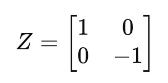
  • Z Gate: The Pauli-Z gate introduces a phase flip, changing the phase of the qubit without altering its state in the computational basis. The matrix representation of the Z gate is:
    z-gate

These gates are fundamental operations in quantum computing, and they are used in various algorithms to manipulate qubit states.

3.2 Hadamard Gate (H)

The Hadamard gate is one of the most important gates in quantum computing because it creates superposition. When applied to a qubit in the state |0โŸฉ, it transforms the qubit into an equal superposition of |0โŸฉ and |1โŸฉ. When applied to a qubit in the state |1โŸฉ, it creates a superposition of |1โŸฉ and |0โŸฉ.

The matrix representation of the Hadamard gate is:
h-gate

The Hadamard gate is critical for algorithms such as Groverโ€™s search algorithm and Shorโ€™s factoring algorithm, where it is used to create superpositions of different states that explore multiple possibilities simultaneously.

3.3 Phase Gates (S, T)

Phase gates are used to add a phase shift to the quantum state of a qubit.

  • S Gate: The S gate, also known as the phase gate, applies a phase of ฯ€/2 to the qubit, shifting the phase of the |1โŸฉ state by 90 degrees. The matrix representation of the S gate is:
    s-gate
  • T Gate: The T gate applies a phase of ฯ€/4 to the |1โŸฉ state, introducing a smaller phase shift than the S gate. The matrix representation of the T gate is:

Phase gates are used in quantum algorithms for introducing relative phase shifts between quantum states, a key component for interference effects in quantum circuits.

3.4 CNOT Gate

The Controlled-NOT (CNOT) gate is a two-qubit gate that performs a NOT operation on the second qubit (the target qubit) only if the first qubit (the control qubit) is in the |1โŸฉ state. This gate is the foundation for creating entanglement between qubits.

The matrix representation of the CNOT gate is:
cnot-gate

The CNOT gate is used extensively in quantum algorithms and quantum error correction, where it helps to create entangled states.

3.5 Toffoli Gate (CCNOT)

The Toffoli gate, also known as the controlled-controlled-NOT (CCNOT) gate, is a three-qubit gate that flips the third qubit (the target qubit) if and only if both the first and second qubits (the control qubits) are in the |1โŸฉ state.

The matrix representation of the Toffoli gate is:
ccnot-gate

This gate is useful in reversible computing and error correction protocols.

3.6 SWAP Gate

The SWAP gate exchanges the states of two qubits. It is a two-qubit operation that swaps the quantum states between two qubits.

The matrix representation of the SWAP gate is:
swap-gate

The SWAP gate is important in quantum circuits for reordering qubits and in quantum error correction.

3.7 Controlled-Phase (CPHASE) Gate

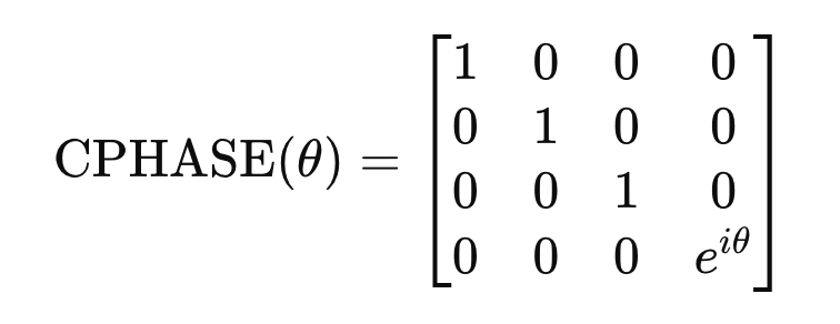
The Controlled-Phase (CPHASE) gate introduces a phase shift between the target qubit and control qubit when the control qubit is in the |1โŸฉ state. The matrix representation of the CPHASE gate is:
cphase-gate

3.8 Rotation Gates (Rx, Ry, Rz)

Rotation gates are used to rotate qubits around specific axes of the Bloch sphere. The rotation gates Rx, Ry, and Rz apply rotations around the X, Y, and Z axes, respectively.

  • Rx Gate: Applies a rotation around the X-axis.
  • Ry Gate: Applies a rotation around the Y-axis.
  • Rz Gate: Applies a rotation around the Z-axis.

Each of these gates has a corresponding matrix representation, and they are used in quantum algorithms to modify the states of qubits by specific angles.


4. Quantum Circuit Representation

A quantum circuit is made up of quantum gates that are applied to qubits. These circuits are represented visually as a sequence of gates on horizontal lines representing qubits. A quantum circuit diagram shows the qubits as horizontal lines, and gates are applied to them as symbols placed on these lines.

Quantum circuits can be simulated and executed using platforms like Qiskit, where quantum gates are represented using the QuantumCircuit class.


5. Quantum Gate Operations: Superposition, Entanglement, and Interference

Quantum gates manipulate quantum states by performing operations like creating superposition (Hadamard gate), introducing entanglement (CNOT gate), and controlling phase shifts (Phase gates). These operations leverage the principles of quantum mechanics, enabling quantum computers to perform tasks that are infeasible for classical computers.


6. The Matrix Representation of Quantum Gates

Quantum gates are described using matrices because quantum states are vectors, and gates are linear operations on these vectors. The unitary matrix representation ensures that the probability amplitudes are preserved (i.e., the system’s total probability is always equal to 1).


7. How Quantum Gates Are Used in Quantum Algorithms

Quantum gates are used to build quantum algorithms like Grover’s search algorithm, Shor’s factoring algorithm, and quantum teleportation. These algorithms exploit the unique properties of quantum gates to solve problems much faster than classical computers.


8. Implementing Quantum Gates Using Qiskit

Qiskit is a Python library that allows you to create, simulate, and run quantum circuits. Implementing quantum gates in Qiskit involves defining quantum circuits and using built-in methods for applying gates like circuit.h(0) for the Hadamard gate or circuit.cx(0, 1) for the CNOT gate.


9. Quantum Gates and Quantum Error Correction

Quantum gates also play a role in quantum error correction. Error correction codes like the Shor code and the Steane code use quantum gates to detect and correct errors that arise from noise during quantum computations.


10. Advanced Quantum Gates and Their Applications

Advanced quantum gates like the Toffoli gate and the Fredkin gate have applications in quantum reversible computing and quantum cryptography.


11. Quantum Gate Visualization Tools

Several visualization tools, such as Bloch sphere representations and quantum circuit simulators, allow researchers and learners to see how quantum gates affect quantum states visually.


12. Resources for Further Learning

To learn more about quantum gates, quantum computing, and related topics, the following resources are recommended:

  • Qiskit Documentation: Official documentation for Qiskit, which is widely used for quantum computing experiments.
  • Quantum Computation and Quantum Information by Michael Nielsen and Isaac Chuang: A comprehensive textbook for quantum computing.
  • IBM Quantum Experience: A platform for learning and experimenting with quantum circuits using actual quantum hardware.

13. Conclusion

Quantum gates are fundamental to the operation of quantum computers. They allow quantum states to be manipulated in ways that classical gates cannot achieve, thanks to the unique properties of quantum mechanics like superposition and entanglement. As quantum computing continues to evolve, the understanding and application of quantum gates will remain at the forefront of innovation in this exciting field.